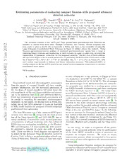
Estimating parameters of coalescing compact binaries with proposed advanced detector networks

0.59 MB·English

by  J. Veitch

Estimating parameters of coalescing compact binaries with proposed advanced
detector networks
J. Veitch,1,∗ I. Mandel,2,3,† B. Aylott,3 B. Farr,4 V. Raymond,4
C. Rodriguez,4 M. van der Sluys,5 V. Kalogera,4 and A. Vecchio3
1School of Physics and Astronomy, Cardiff University, 5, The Parade, Cardiff, UK, CF24 3YB
2NSF Astronomy and Astrophysics Postdoctoral Fellow, MIT Kavli Institute, Cambridge, MA 02139
3School of Physics and Astronomy, University of Birmingham, Edgbaston, Birmingham, B15 2TT
4Center for Interdisciplinary Exploration and Research in Astrophysics (CIERA) & Dept. of Physics and Astronomy,
Northwestern University, 2145 Sheridan Rd, Evanston, IL 60208, USA
5Radboud University Nijmegen, P.O. Box 9010, NL-6500 GL Nijmegen, The Netherlands
(Dated: January 6, 2012)
The advanced versions of the LIGO and Virgo ground-based gravitational-wave detectors are
2 expected to operate from three sites: Hanford, Livingston, and Cascina. Recent proposals have
1 been made to place a fourth site in Australia or India; and there is the possibility of using the
0
Large Cryogenic Gravitational Wave Telescope in Japan to further extend the network. Using
2
Bayesian parameter-estimation analyses of simulated gravitational-wave signals from a range of

n coalescing-binary locations and orientations at fixed distance or signal-to-noise ratio, we study the
a improvement in parameter estimation for the proposed networks. We find that a fourth detector
J sitecanbreakdegeneraciesinseveralparameters;inparticular,thelocalizationofthesourceonthe

5 sky is improved by a factor of ∼ 3–4 for an Australian site, or ∼ 2.5–3.5 for an Indian site, with
more modest improvements in distance and binary inclination estimates. This enhanced ability to

] localizesourcesontheskywillbecrucialinanysearchforelectromagneticcounterpartstodetected
E
gravitational-wave signals.
H
. PACSnumbers:
h
p
- I. INTRODUCTION to add a fourth site to the network, at Gingin in West-
o
ern Australia (- 31◦21(cid:48)28(cid:48)(cid:48) S, 115◦42(cid:48)50(cid:48)(cid:48) E) , or outside
r
t BangaloreinIndia(14◦14(cid:48) N,76◦26(cid:48) E).Theadvantages
s Gravitational waves and electromagnetic counterparts
a and disadvantages of the LIGO Australia and LIGO In-
from the merger of compact binaries will carry comple-
[ dia proposals were studied by a working group within
mentary information, and the successful association of
the LIGO Scientific Collaboration, and their conclusions
1
the two types of merger signatures will allow many cru-
v for LIGO Australia reported in [8]. The Large Cryo-
cialquestionsinstellarandbinaryevolutionandcosmol-
5 genicGravitationalWaveTelescope(LCGT)detectorisa
ogy to be answered (see [1, 2] and references therein).
9 plannedinterferometerwith3kmarmsandcryogenically
1 Good sky localization of gravitational-wave sources will cooled mirrors, located in Japan (36◦15(cid:48) N, 137◦11(cid:48) E)
1 be crucial in searching for associated electromagnetic
200 metres below ground to reduce seismic noise [9]. In
. transients. In this paper, we discuss ways in which relo-
1 addition to the 4-site advanced LIGO/Virgo networks,
cating one of the LIGO detectors to a site in Australia
0 wealsoconsiderthepossiblenetworkwithtwoadvanced
2 or India could improve the prospects of multi-messenger LIGOdetectorsatHanford,oneatLivingston; advanced
1 gravitational-wave astronomy.
Virgo at Cascina and LCGT in Japan. In the following,
:
v The final S6 science run of the enhanced-LIGO gravi- weuseanacronymfordenotingthenetworkbasedonthe
i tational wave detectors [3], along with the third science first initials of the sites involved: Australia (A), Hanford
X
run of the Virgo detector [4] and GEO 600 [5], has re- (H), India (I), Japan (J), Livingston (L) and Virgo (V);
r
a cently concluded. Construction of the second generation e.g., AHLV is a network consisting of LIGO detectors in
of instruments is already underway, with 4km Advanced Australia, Hanford and Livingston and the Virgo detec-
LIGO detectors undergoing installation at the Hanford, tor.
WA and Livingston, LA observatories [6], with sensitiv-
In this study, we make a comparison of the perfor-
ity expected to improve by about one order of magni-
mance of the proposed networks with the performance
tude. These two sites in North America are expected to
of the 3-site HHLV network in terms of parameter es-
be joined by the Advanced Virgo [7] detector, located in
timation for compact binaries. We focus on binary
Cascina, Italy, to form a second-generation network con-
neutron-star systems, which are expected to be a preva-
sistingofthreesites. Recently,proposalshavebeenmade
lentsourceofobservablesignalsfortheadvanceddetector
network [10].
Using independent Bayesian analyses, we compare the
∗Electronicaddress: [email protected] parameterestimationperformanceofeachnetworkforan
†Electronicaddress: [email protected] ensemble of sources spread throughout parameter space,
2
and demonstrate the improvement gained from the ad- II. NETWORK CONFIGURATIONS
dition of sites to the network. The relative improve-
ment for individual sources is assessed at a fixed dis-
Interferometricgravitationalwavedetectorsarenotori-
tance or signal-to-noise ratio. Bayesian inference allows
ouslybadatdeterminingthedirectionofincomingradia-
us to extract all of the available information about sys-
tion from short duration sources when used individually,
tem parameters from the full data set. In contrast with
as the detector has good sensitivity over a large range
the timing triangulation method discussed below, all of
of angles. Although this allows an all-sky search to be
the data from all interferometers are taken into account
performed without the need for ‘pointing’, it also means
coherently. And unlike Fisher information matrix tech-
thattheamplitudeoftheincomingsignalcannotbeused
niques, which explicitly only describe the local structure
to determine its location well. To be able to resolve the
oftheparameterspaceandareaccurateonlyinthelimit
positionontheskyofashortdurationgravitationalwave
of high signal-to-noise ratio (SNR), Bayesian inference
source, a network of interferometers is needed.
methods search through the full parameter space, show-
With more than one site it is possible to use triangu-
ing the global structure of posteriors, including multiple
lationtodeterminethelocationofanobservedsignalus-
modes or near-degeneracies.
ing the observed time delay between different detectors.
Beginning with the work of [11], several other stud- With two sites, this method can resolve the position to
ieshaveanalyzedsky-localizationaccuracywithdifferent within a ring on the sky centered on the axes between
network configurations [12–15]. These investigations ei- the sites; with three sites this is reduced to two patches;
therusedonlyalimitedamountofinformation(e.g.,tim- but the addition of a fourth site allows a unique patch
ing information alone) or Fisher-matrix techniques that tobedeterminedforeachsource. Thelimitingfactorsin
may fail in a multimodal, degenerate parameter space. the accuracy of the timing method are the distances be-
ThestudybyNissankeet al. [16]usedBayesianmethods tweenthesitesinthenetworkandthetimingaccuracyof
to compare HLV, AHLV, HJLV and AHJLV networks, the sites, which is itself governed by the signal-to-noise
but used a single detector at Hanford for the HLV case ratio and the effective bandwidth of the signal in each
(so some of their quoted improvements are simply due detector [12]. So, to achieve a better sky resolution for
to greater SNR accessible with 4 rather than 3 detec- any particular gravitational wave, a network should con-
tors). Furthermore, [16] used a population of sources sistofdetectorswithawidebandofsensitivity, withthe
randomly distributed in space out to z = 1, whereas we longest possible baselines between sites. As the sensitive
distributed our sources at constant distance (for nested band of the noise curve is generally limited by available
sampling [NS] and Markov Chain Monte Carlo [MCMC] technology and fundamental noise sources, we are left
methods) or constant SNR (Fisher matrix method) and with the option of dispersing the detectors as widely as
varied the other extrinsic parameters. This was done possible.
to ensure good coverage of the extrinsic parameter space Given the necessity to build detectors on Earth, the
whenassessingtherelativenetworkperformances. Mean- maximumpossiblebaselinewouldbethediameterofthe
while,thestudybyKlimenkoet al. focusedonskylocal- Earth,42.5ms(distancesconvertedtogravitational-wave
ization of transient burst sources rather than coalescing travel times). The existing LIGO-Virgo network of de-
compact binaries with known waveforms [17]. tectorsconsistsofthreesites,atHanford,Livingstonand
The “Report of the Committee to Compare the Sci- Cascina, all in the northern hemisphere. The longest
entific Cases for AHLV and HHLV”, which considered baseline between detectors in this network, Hanford-
the scientific advantages of moving one of the Hanford Virgo, is 27ms. With the addition of the Gingin site to
detectors to Australia [8], was based in part on a pre- thenetwork,thisisincreasedto41msfortheLivingston-
liminary version of the work presented here. Ours is the Gingin baseline, close to the maximum possible, and the
first study to apply Bayesian techniques to comparisons two baselines from Gingin to the other sites are all also
of parameter-estimation accuracies with a network in- of great length. The Japanese and Indian sites similarly
cludinganIndiandetectoraswellasnetworkswithAus- increase the longest baseline, with Japan being closer to
tralian or Japanese detectors. Furthermore, we analyze the U.S. sites but India closer to Virgo. All times are
the impact of moving one of the detectors to Australia given for reference in table I.
or India on the accuracy of measuring masses, distances, In this study, we compare the networks under the as-
and other parameters in addition to sky localization for sumptionthatalldetectorsareoperationalatthetimeof
the first time [41]. the observation of a signal. In practice, however, detec-
Thispaperisorganizedasfollows. InsectionII,wede- torshavelimiteddutyfactors. Theprobabilityofhaving
scribethenetworkconfigurationsbeinganalyzed. Insec- at least three non-colocated detectors up at a given time
tion III, we introduce the analysis techniques employed is higher with the larger networks than with the HHLV
in this paper. The simulations and their results are de- network, increasing the probability for decent source lo-
scribed in section IV. We conclude in section V. We also calization.
include an appendix discussing the impact of the change Although the triangulation method above captures
ofnetworkconfigurationsonfalsealarmprobabilitiesand well the essential reason for desiring a longer baseline,
detection thresholds for a fully coherent analysis. the methods used in this paper are based on a fully co-
3
H L V A I J model hypothesis H, which is
H 0 10 27 39 36 25
p(θ(cid:126)|H)p(d˜|θ(cid:126),H)
L 10 0 26 41 39 32 p(θ(cid:126)|d˜,H)=
p(d˜|H)
V 27 26 0 37 22 29
(cid:18) (cid:19)
1
A 39 41 37 0 14 7 ∝p(θ(cid:126)|H)exp − (cid:104)d˜−h˜(θ(cid:126))|d˜−h˜(θ(cid:126))(cid:105) ,
2
I 36 39 22 14 0 21
(3.1)
J 25 32 29 7 21 0
TABLE I: Table of gravitational-wave travel times between where p(θ(cid:126)|H) is the prior probability density of the pa-
sites (Hanford, Livingston, Virgo, Australia, India, Japan, rameters θ(cid:126) and h˜(θ(cid:126)) is the model used to describe the
identified by their first letters), in milliseconds. The maxi- signal in the frequency domain [25]. The noise-weighted
mum possible baseline for a terrestrial network is 42.5ms.
residuals in the presence of Gaussian noise with power
spectral density S (f) are given by
n
(cid:12) (cid:12)2
herent Bayesian analysis of the data to extract posterior (cid:90) ∞ (cid:12)(cid:12)d˜(f)−h˜(f;θ(cid:126))(cid:12)(cid:12)
probability functions on the parameters of interest. This (cid:104)d˜−h˜(θ(cid:126))|d˜−h˜(θ(cid:126))(cid:105)=4 df. (3.2)
S (f)
method naturally incorporates the information from the 0 n
time delays between sites, but it also includes the infor- For these simulations, for the LIGO and Virgo detec-
mation from the amplitudes and relative phases of the tors,includingtheAandIsites,weusedsimulatednoise
signalspresentineachdetector. Thisinformationcanbe with noise power spectral density S (f) similar to the
n
used to further restrict the sky location, for example by Advanced LIGO design curve from the LIGO Algorithm
eliminating the secondary maximum in the sky location Library (LAL) [26]. Use of the Advanced LIGO noise
for the majority of signals in the 3-detector network. curve for the Advanced Virgo detector may change the
The addition to the network of a fourth site also gives absolute results slightly, however the relative improve-
a fourth separate detector orientation (instead of the ments ought to be consistent. The noise curve fit has a
replica of the H1 detector in the HHLV network). This functional form of
raises the possibility of improved measurement of the (cid:40)(cid:18)f (cid:19)−4.14 (cid:18)f (cid:19)2
other parameters of the source, in particular, the mea- S (f)=S −5 0
surement of the polarization angle ψ and inclination an- n 0 f0 f
gle ι of the gravitational wave may be expected to im-  (cid:16) (cid:17)2 (cid:16) (cid:17)4
ppraorviseoinnocfemrteaainsucraesmese.nWtaecpcuerrfaocrimesaofctohmespereahnednsoitvheecropma-- +1111− ff0 (cid:16)+ 12(cid:17)2ff0 , (3.3)
rameters encoded in the gravitational-wave signal from 1+ 1 f 
2 f0
an inspiraling binary composed of non-spinning neutron
stars. where S = 1049Hz−1 and f = 215Hz. For the LCGT
0 0
detector, an interpolated LCGT design sensitivity curve
was used [9, 27].
TheMCMCmethodusedbyLALInferenceMCMC ex-
plores the parameter space with a random walk, using
III. ANALYSES the Metropolis-Hastings algorithm to simulate samples
θ(cid:126) from the posterior probability distribution function
p(θ(cid:126)|d,H). LALInferenceMCMC uses a variety of op-
For this study, we used two independent Bayesian in-
timisation techniques, including parallel tempering, to
ference codes that implement two different techniques:
convergeonthemodesofthedistributionandensuread-
the LALInferenceMCMC code (based on the SPINspi-
equate mixing of the chain [18–20]. It was started with
ral code [18–20]) uses a Markov Chain Monte Carlo al-
randomly offset parameter values to simulate imperfect
gorithm (MCMC) [21], while the Inspnest code [22, 23]
initial inputs from the detection pipeline, and 10 chains
uses nested sampling [24].
ran on each event to check for convergence.
Both techniques stochastically sample the parameter ThenestedsamplingalgorithmusedbyInspnest oper-
space in a search for the parameters that best match the ates by generating and replacing samples from the prior
observed data, simultaneously finding the set of param- distribution p(θ(cid:126)), gradually shrinking the volume sam-
eters that yield the best fit to the data, and determin- pledbyimposingalimitofminimumlikelihoodp(d|θ(cid:126),H)
ing the accuracy of the parameter estimation. This is on each replacement sample [24]. Inspnest samples the
achieved by calculating the posterior probability density prior distribution using an MCMC algorithm, which is
function (PDF) on the parameter space θ(cid:126) of the signal, optimisedforexploringthestructureofthelimitedprior,
given the data in the frequency domain d˜, and a signal with jumps proposed through differential evolution, and
4
along possible degeneracies in parameter space [22, 23]. pNorder(see, e.g., [31,32]foradditionalinformationon
It is designed to compute the evidence p(d|H), but the post-Newtonian waveform approximants).
outputsamplesfromthepriorcanbeweightedappropri-
Injections were coherently made into four network
ately and resampled to produce samples from the poste-
configurations: (i) HHLV, (ii) AHLV, (iii) HILV, (iv)
rior distribution.
HHJLV. All injections were performed using Gaussian
The output from both Bayesian codes is a list of sam-
colored noise, using the Advanced LIGO power spec-
ples from the posterior distribution p(θ(cid:126)|d,h), which are tral density approximated by Eq. (3.3) for the Advanced
thenusedtoestimatethemean,variance,andpercentiles LIGOandAdvancedVirgosites(includingAustraliaand
of the distributions. We performed two-dimensional India),andafittotheLCGTnoisecurvefortheJdetec-
binning and used a greedy algorithm to compute two- tor in the HHJLV network. In each of the four-site net-
dimensional minimum probability intervals, as explained works the noise realizations were kept the same in each
in section IV. network, although the sites are moved. In the HHJLV
AswellasthetwoBayesianmethods, wealsousedthe network the noise realisation in the HHLV portion was
Fisher information matrix (FIM) to estimate the mea- the same as in the other 4-site networks. We also exam-
surement uncertainties. The FIM technique, which ap- ined the possibility of rotating the Australia detector by
proximates the likelihood surface quadratically near the 45◦, and found very similar results to the AHLV case,
likelihood peak, has a long history in gravitational-wave which are omitted from further discussion for brevity.
parameter estimation (e.g., [28]). It is known to suf-
The additional A and I detectors were positioned with
fer from a number of flaws, particularly in the low-SNR
their arms oriented along the local North and East vec-
limit (when the quadratic approximation breaks down),
tors projected onto the tangent plane to the Earth’s sur-
or when correlations between parameters are very signif-
face at the site, whose locations are given in section I.
icant [29]. Furthermore, the Fisher information matrix
The J detector was aligned with its y-arm 19◦ from the
is entirely local, and only approximates the shape of the
localNorthvectorasthegeometryofthedetectoriscon-
maximum where it is evaluated, ignoring other maxima
strained by the existing underground tunnels.
intheglobalparameterspacewhicharepickedupbythe
Bayesian analyses. On the other hand, the FIM tech- As the speeds of the methods differed, we performed a
nique is computationally inexpensive, and hence allows different set of simulations with each method, with the
a larger number of sources to be simulated in order to following details.
improve statistics.
The signal model for a non-spinning inspiral signal re-
quires nine physical parameters: the chirp mass M =
(m m )3/5(m + m )−1/5 and the symmetric mass ra-
1 2 1 2 Nested Sampling
tio η = m m (m +m )−2 (where m and m are the
1 2 1 2 1 2
individualmasses),rightascensionα,declinationδ,incli-
nation ι, orientation ψ, the luminosity distance d , the The nested sampling implementation was able to run
L
time of coalescence t and the phase at coalescence φ. on a large set of injections. All signals were injected at a
c
For the Bayesian analyses, the prior probability distri- luminosity distance of 180 Mpc, but the inclination an-
bution was assumed to be isotropic on the sphere of the gle, polarization angle, right ascension and declination
sky, and on the inclination of the binary relative to the were located on a 5×6×5×5 rectangular grid in the
line of sight, and proportional to d 2. All other priors α× sinδ× cosι×ψ parameter space for a total of 750
L
are uniform unless otherwise specified. injections. This resulted in a range of SNRs between 5
and 35, but mostly between 7 and 25. We chose low
and high frequency cutoffs of 30Hz and 2048Hz, which
included the maximum frequency of the inspiral signal
IV. SIMULATIONS
as no merger or ring-down components were used. Of
the 750 signals, 728 were detected in all network con-
For this study, we assumed that a successful detection
figurations, and it is these we will use for the summary
has already been made, and we have the correct wave-
statistics throughout the remainder of the paper. The
form model to process the data, so we did not perform
nested sampling search, by its nature, samples the entire
evidence calculations or model selection. The waveform
prior range given for the parameters. In this case, the
model used for injection in all cases was generated by
total mass M = m +m was assumed to be between
the LIGO Algorithm Library GeneratePPNInspiral rou- 1 2
2 and 35 M , with component masses allowed to be in
tine [26], which uses a time-domain approximant at 2.0 (cid:12)
therangem ,m ∈[1,30]M . Thepriordistributionon
pN order in phase and 0 pN order in amplitude [30]. 1 2 (cid:12)
M used was p(M) ∝ d2M−5/6, chosen as an approx-
All injections used symmetric binary neutron star sig- L
imation to the Jeffrey’s prior which sets the prior as a
nals with masses m = m = 1.4M as observed in
1 2 (cid:12) function of the Fisher matrix Γ on the parameter space,
the detector frame. For recovery and posterior calcu- (cid:113)
lation, we used the frequency-domain stationary phase p(θ(cid:126)) ∝ detΓ(θ(cid:126)), in order to improve sampling where
approximation TaylorF2 approximant from LAL at 2.0 the template bank density is highest [33].
5
MCMC F < 1, the F-width of a one-dimensional PDF was
defined as the width of the smallest region that con-
The MCMC method was used to run on a randomly tains that fraction F of the posterior PDF. Thus, the
chosen subset of the injections that were analyzed with 95% width represents the width of the smallest region
nestedsampling(computationalconstraintspreventedus of parameter space that contains 95% of the total pos-
from using the full set of injections). Results from 42 in- terior probability. A similar approach was used for two-
jections are used in this analysis. For consistency, the dimensional PDFs in (inclination, distance) space and
MCMC runs employed the same priors and frequency (rightascension,declination)space,withpixelsofafixed
rangefortheoverlapintegralasthenestedsamplingruns. size (0.25 deg2) being used in a greedy algorithm to esti-
TheMCMCresults onindividualinjectionsmatchedthe mate the sky area for sky localization.
nested sampling results, therefore allowing us to gain Wealsodefinea“standardaccuracy”(byanalogywith
extra confidence in the Bayesian parameter estimation. thestandarddeviation)asthesquarerootofthemeanof
However, because of the concern that smaller numbers the sum of the squared differences between the points in
of runs could increase statistical fluctuations, we do not the PDF (sampled according to the posterior) and the
quoteabsoluteaccuraciesforMCMCruns,butonlycom- true value. Thus, for a marginalized one-dimensional
pare the expected parameter estimation accuracies for PDF,
different network configurations.
(cid:118)
(cid:117) N
(cid:117) 1 (cid:88)
standard accuracy =(cid:116) (x −x )2.
N i true
Fisher Matrix
i=1
The FIM has the advantage of being computationally For a PDF whose mean is equal to the true value, the
inexpensive, and so permits a large Monte Carlo over in- standard accuracy is just the standard deviation. For
jections. Therefore, we used the FIM to confirm the re- a delta-function PDF that is biased away from the true
sults of our Bayesian analyses. We used a low-frequency value, the standard accuracy is the error. In general, the
cutoffof30Hzandintegrateduptotheinnermoststable standard accuracy is equal to the sum, in quadrature,
circular orbit frequency, around 1600 Hz. of the standard deviation of the PDF and the difference
For this study, we varied all angles in a Monte Carlo between the PDF mean and the true value.
of 4000 points, adjusting the distance to keep the total
network SNR equal to 30 for all injections in all network
configurations. We chose injections with this relatively B. Relative Improvements
highvalueofSNR,ratherthantheSNRdistributionused
for nested sampling and MCMC studies, because of con-
Inthefollowingsections,wepresenttheresultsofeach
cernsaboutthetheaccuracyoftheFIMapproachoutside
of the three analyses of the differences in parameter es-
the high-SNR limit. The SNRs were separately normal-
timation accuracy between the three networks. In the
ized to 30 for all networks, including the five-detector
caseofthetwoBayesiancodes,wemeasurethe95%con-
HHJLVnetwork; therefore,resultsforthatnetworkfrom
fidence intervals for each parameterand compute the ra-
the FIM study are expected to be worse than those ob-
tio of these in comparison to the result from the HHLV
tainedwithBayesianstudies,whichwouldnormallyhave
network for the same injection. The median value of the
higher SNRs in the five-detector network than the four-
ratio is quoted in each table, along with the range incor-
detector networks for a given injection.
porating the 5% and 95% quantiles of the distribution.
Thisgivessomemeasureofthespreadoftheratiosacross
different sky positions, locations and orientations.
A. Quantities compared
Although our techniques make full nine-dimensional
posterior PDFs available, these are unwieldy to compare MCMC results
or visualize. So we typically consider only one- or two-
dimensional PDFs marginalized over the remaining pa- In table II, we average comparisons of the 95% con-
rameters, with examples shown in figures 4 & 3. How- fidence intervals across the 42 injections analyzed with
ever,toallowustomakecomparisons,wehadtorestrict the LALInferenceMCMC code. We show the values of
ourselvestoparticularestimatorsforthePDFs,withthe the 95% confidence interval widths for the extended net-
understanding that unless PDFs are extremely narrow work configurations as fractions of the same widths for
or are described by a simple analytical function (e.g., a the HHLV configuration. Table II lists the median ratio
Gaussian), afewestimatorsarenotsufficienttodescribe of the size of the 95% probability region over all of our
all of the information contained in the PDFs. injection runs, while the 5% and 95% percentiles of the
We estimated the width of a particular one- or two- distribution of ratios are shown in super and subscript,
dimensional PDF as follows. For a given fraction 0 < to indicate the range of the results.
6
AHLV / HHLV HILV / HHLV HHJLV / HHLV
Parameter 95% width std. acc 95% width std. acc 95% width std. acc
M 0.97+2.03 0.93+2.59 1.00+2.18 0.85+2.27 0.82+1.92 0.72+3.23
−0.66 −0.66 −0.65 −0.73 −0.80 −0.69
η 0.93+3.27 0.94+3.34 0.96+1.26 0.80+1.63 0.88+1.72 0.77+3.61
−0.70 −0.80 −0.59 −0.55 −0.63 −0.50
t 0.62+1.06 0.46+1.02 0.71+1.86 0.62+1.22 0.55+0.60 0.37+1.98
c −0.47 −0.41 −0.51 −0.56 −0.42 −0.32
d 0.93+0.29 0.98+0.11 0.93+0.38 0.96+0.17 0.85+0.40 0.95+0.19
L −0.23 −0.36 −0.24 −0.35 −0.27 −0.33
α 0.50+1.23 0.43+0.77 0.59+0.53 0.47+1.87 0.50+0.83 0.46+1.47
−0.29 −0.41 −0.46 −0.45 −0.43 −0.44
δ 0.43+0.74 0.27+0.98 0.50+0.70 0.46+0.97 0.55+0.62 0.29+1.67
−0.35 −0.23 −0.38 −0.43 −0.42 −0.24
ι 0.85+0.51 1.01+0.64 0.88+0.42 1.00+0.35 0.82+0.68 1.04+0.54
−0.31 −0.56 −0.52 −0.41 −0.45 −0.47
ψ 0.98+0.38 0.98+0.16 0.97+0.38 0.99+0.11 0.95+0.55 0.99+0.17
−0.60 −0.17 −0.66 −0.25 −0.63 −0.15
α−δ 0.27+0.65 — 0.30+0.89 — 0.38+0.77 —
−0.21 −0.22 −0.29
d −ι 0.76+0.49 — 0.80+0.36 — 0.76+0.57 —
L −0.32 −0.54 −0.51
TABLE II: Comparative 95% interval widths and standard accuracies for one-dimensional PDFs, and comparative 95% areas
for two-dimensional PDFs (last two lines) averaged over all injections, calculated using the MCMC algorithm. All values are
reported as fractions of the corresponding values for the HHLV network configuration. The median values of the ratios across
all injections are computed; the error bars correspond to the spread between the 5% and 95% quantile values of these ratios
across all injections. See text for details.
AHLV / HHLV HILV / HHLV HHJLV / HHLV
Parameter 95% width std. acc 95% width std. acc 95% width std. acc
M 1.00+0.80 1.00+1.92 1.00+0.71 1.02+1.39 0.92+0.33 0.98+0.34
−0.40 −0.56 −0.47 −0.68 −0.37 −0.42
η 1.00+0.78 1.02+1.28 1.00+0.70 1.01+1.14 0.92+0.30 0.98+0.35
−0.38 −0.51 −0.44 −0.56 −0.29 −0.38
t 0.73+0.54 0.69+1.04 0.69+0.61 0.62+0.90 0.68+0.32 0.66+0.49
c −0.47 −0.61 −0.46 −0.52 −0.43 −0.57
d 1.00+0.33 0.98+0.15 1.05+0.45 0.91+0.53 0.92+0.25 0.98+0.16
L −0.21 −0.25 −0.30 −0.30 −0.24 −0.30
α 0.67+0.58 0.61+0.88 0.62+0.52 0.56+1.00 0.60+0.40 0.56+0.59
−0.48 −0.55 −0.47 −0.50 −0.44 −0.52
δ 0.50+0.70 0.39+1.12 0.61+0.59 0.48+1.02 0.67+0.33 0.59+0.53
−0.40 −0.34 −0.48 −0.41 −0.49 −0.49
ι 0.93+0.24 0.91+0.35 0.86+0.28 0.83+0.56 0.86+0.19 0.90+0.26
−0.46 −0.58 −0.47 −0.56 −0.44 −0.59
ψ 1.00+0.19 0.99+0.32 0.97+0.11 0.91+0.32 0.93+0.11 0.97+0.22
−0.52 −0.51 −0.66 −0.63 −0.52 −0.56
α−δ 0.32+0.78 — 0.43+0.87 — 0.33+0.51 —
−0.24 −0.32 −0.22
d −ι 0.90+0.29 — 0.88+0.44 — 0.53+0.24 —
L −0.45 −0.49 −0.27
TABLE III: Comparative 95% probability interval widths and standard accuracies between alternative network configurations
andtheHHLVnetwork,calculatedusingthenestedsamplingalgorithm. Themedianvaluesoftheratiosacross728injections
detected in all networks are computed. Errors quoted correspond to the 5% and 95% quantiles of the distribution of ratios, as
in table II. For α−δ plane, 95% probability intervals are calculated using a greedy binning algorithm.
Parameter AHLV/HHLV HILV/HHLV HHJLV/HHLV
M 1.00 1.00 1.02
η 1.00 1.00 1.02
t (msec) 0.54 0.56 0.65
c
d 0.77 0.66 0.71
L
α (deg) 0.66 0.56 0.50
δ (deg) 0.31 0.57 0.62
ι (deg) 0.76 0.67 0.70
ψ (deg) 0.77 0.67 0.69
φ (deg) 0.88 0.84 0.91
c
α−δ (deg2) 0.29 0.35 0.47
TABLE IV: Ratios of median standard deviations for each parameter and the sky area as reported by the Fisher information
matrix, as a function of network configuration. All injections are re-normalized to an SNR of 30 in the given network, so the
last column, corresponding to a five-detector network re-normalized to the same SNR as the four-detector networks, can not
be directly compared to similar columns in the tables above.
As discussed in more detail below, the accuracy with cantly affected by the network configuration. This con-
which individual masses can be recovered is not signifi- formstoourexpectationthatmassmeasurements,which
7
1 forrelativetimingmeasurements. Thegreatestimprove-
ment is seen for the addition of the the Australian de-
n0.8 tector, yielding the longest north-south baseline. HILV
o
cti and HHJLV are both great improvements on the HHLV
e fra0.6 AHLV network, and have similar performance for the majority
v of signals, although HHJLV suffers from fewer outliers
ulati0.4 HHLV withskyresolutiongreaterthan100squaredegrees,pos-
m HILV sibly due to the increased signal-to-noise ratio from the
u
C0.2 HHJLV additional detector.
Thisimprovedperformanceisreflectedinthecompari-
0 sonofthemedian95%confidenceintervalforeachofthe
100 101 102 103
networks, given intable V.The medianresolutionfor all
Probability interval (square deg)
sourcesshrinksfrom30.25squaredegreesto6.625square
degreesbetweenHHLVandthemostaccurateAHLVnet-
FIG.1: Cumulativehistogramofthe95%confidenceinterval
fortheareaoftheskyinsquaredegrees,estimatedusingthe work. In addition to the reduction of the median resolu-
Inspnest analysisof728signalswhichweredetectedinallnet- tion,theseimprovementsarealsoreflectedintherelative
work configurations, covering the range of sky locations and resolutions of the networks. Table III shows the median
orientationsofthebinary. Differentlinescorrespondtodiffer- ratio of the 95% probability region size for the extended
ent networks: green dot-dashed line, AHLV; red dashed line, networks against HHLV; note that the median of the ra-
HHLV;cyansolidline,HILV;blacksolidlineHHJLV.Theex- tios for the sky location intervals (α−δ row) is not the
tended networks show significantly better performance than
same as the ratio of the medians in table V.
the3-sitenetwork,withAHLVofferingthehighestfractionof
The qualitative behavior inferred from the LALInfer-
signals resolved to better than 10 square degrees. HILV and
enceMCMC andInspnest runsisinexcellentagreement.
HHJLV show similar performance to each other for a large
fraction of the signals, but the HHJLV network avoids the Some differences between the “typical” results tables III
tailofpoorlyresolvedsignalslocatedinregionsofparameter and II are due to the impact of statistical fluctuations in
space with poor sensitivity in HILV. the smaller subset of injections analyzed with LALInfer-
enceMCMC ; however, we have confirmed quantitative
agreement between the two methods on the individual
come from waveform phasing, are constrained primar- injections being analyzed.
ily by the total network SNR. Sky localization accuracy For a more detailed look at the performance of the
can be significantly improved in both directions when a networks for the non-sky-location parameters, we show
fourth site is added to the network. Timing accuracy at in figure 5 the cumulative probability distributions for
the geocenter is strongly correlated with sky localization the fraction of signals found within a given probability
and is similarly improved. A fourth site also moderately interval width for M, η, d , ι, ψ and t . Although our
L c
improves the accuracy of distance measurements. rangeofinjectionsatconstantdistanceisastrophysically
We should particularly point out the next-to-last line unrealistic, these figures give a good idea of the relative
of the table, “α − δ”. The area of this 2-dimensional performanceofthenetworksacrossanisotropicdistribu-
PDF is a direct measure of the uncertainty in estimat- tion of sky position, polarisation and inclination angles.
ing the position of the source on the sky. The error box Wecanseeimmediatelythattheimprovementintheres-
shrinksbyafactorof∼4whenthesecondHanforddetec- olution of the chirp mass and η parameters is marginal,
tor is moved to Australia or India because of the much- as evident from tables III. The slightly improved perfor-
improvednorth-southbaseline. Thisimprovementinsky manceforHHJLVcanbeattributedtothehighersignal-
localization accuracy will make the detection of an elec- to-noiseratiointhatnetworkthankstothefifthdetector.
tromagneticcounterparttothegravitational-wavesource
With the distance and inclination angle parameters,
morefeasible,andisperhapsthebiggestbooninmoving
we see slight improvements, with the biggest effect again
one of the Hanford detectors to India or Australia.
being produced by the additional SNR in the HHJLV
network. Due to degeneracies in the parameter space,
the effect is more pronounced when the two dimensional
Inspnest results distribution is considered, as in section IVC. From table
III, we see that the median relative improvement of the
In figure 1 we show the results of determining the sky polarizationangleψresolutionisminimal,howeverinfig-
location of 728 injections with the Inspnest nested sam- ure5 itis apparent thatfor the 4-site networks thereare
pling code. The lines show the cumulative histograms a greater fraction of injections which are resolved well.
for the 95% confidence interval on the sky location of Thisisexplainedbythelargefractionofsignals(∼50%)
the binary for each of the network configurations consid- which have a very broad distribution where the ψ pa-
ered. As expected, the addition of a fourth site to the rameter is degenerate with the phase of the signal, when
network yields a significant improvement in the resolu- ι is close to 0 or π. Although the median of the im-
tion of the sky location, due to the increased baseline provement ratio for individual sources is ∼ 1, the mean
8
is ∼ 0.95 for HALV and ∼ 0.85 for HILV and HHJLV,
indicatingthatthesourceswhichcanberesolvedinψare 1.0 FIM Solid Angle Standard Deviations
better resolved in the 4-site networks. The t distribu-
c
tionshowssimilarperformanceforall4-sitenetworksfor
most signals, with slightly fewer signals poorly resolved 0.8
in time with the HILV network than AHLV, reflecting
n
o
the shorter tails of the distributions in figures 1 and 2 acti0.6
(skylocalizationisstronglycorrelatedwiththeaccuracy e fr
of timing the gravitational wave at the geocenter). ativ
mul0.4
u
Network Median 95% conf. int. C
AHLV 6.625 deg2 0.2 AHLV
HHLV
HHLV 30.25 deg2 HHJLV
HILV 9 deg2 HILV
0.0
HHJLV 9.5 deg2 0 2 4 6 8 10
2σ Solid Angle Standard Deviations (deg2)
TABLEV:Median95%confidenceintervalsinsquaredegrees
FIG. 2: A cumulative histogram over injections of the esti-
for each network configuration.
mated accuracies in sky localization obtained via the Fisher
information matrix technique. Blue, green, red and cyan
are the distributions of sky-localization uncertainties for the
AHLV, HHLV, HHJLV and HILV networks, respectively. All
Fisher matrix results
injections are independently normalized to an SNR of 30 for
eachnetworkconfiguration,toavoidconcernsaboutthetrust-
TheFisherinformationmatrixresultsarepresentedin worthiness of FIM results at low SNRs. The relative shapes
table IV. These are ratios of the median standard de- of the histograms are thus more relevant than their actual
viations for each parameter, taken from a Monte Carlo values.
overangles(withdistanceadjustedtokeepthetotalnet-
work SNR equal to 30). According to the FIM results,
the greatest change in sky localization comes from the dimensional estimators used in Tables II, III and IV do
improvement in the measurement of the declination an- not tell the full story because of the strong correlation
gle with a network that includes an Australian detector. between inclination and luminosity distance. The sec-
The declination angle can be measured more accurately ondarymaximumontheskypositionalsocorrespondsto
by a factor of ∼3 with an AHLV network relative to the a secondary mode in the cosι parameter corresponding
HHLVnetwork,asadetectorintheSouthernhemisphere to the transformation ι(cid:55)→π−ι. In fact, the addition of
greatly improves the latitudinal baseline of the network, a fourth site allows this degeneracy to be broken, as can
allowingforsuperiorangularresolutioninthatdirection. be seen by comparing the marginalized one-dimensional
The last line in table IV indicates the Fisher-matrix es- PDFs for a sample injection the HHLV and AHLV net-
timate of the sky area, defined following Eq. (43) of [34]. work configurations, plotted in figure 3. Although the
Figure 2 shows a histogram of the sky-area accuracy for width did not shrink significantly from red to blue pos-
two network configurations. teriors, with the AHLV network configuration the poste-
riors are unimodal and centered on the true values, as a
degeneracy in the inclination-distance space is broken.
C. Parameter Degeneracies Both these effects are clearly visible in figure 4, which
shows the breaking of the degeneracy in d –ι–α–δ space
L
IncaseswhereasignalisobservedwithmarginalSNR asprojectedontothedL–ιandα−δplanes. Inthisexam-
in one or more detectors, or when the orientation of the ple all the expanded networks allow the secondary max-
binary is unfavourable (i.e. ι is close to 90◦), a degen- imum to be eliminated. Figure 6 shows the cumulative
eracy between two sky locations often emerges. The ad- distribution of the 95% probability region for the dL–ι
dition of the fourth site to the network ensures that the space, with the improvement in two dimensions more
source can be localised to a single region on the sky, as prominentthanlookingatdLorιindividually(c.f. figure
shown in the 2-dimensional PDFs of figure 4 which com- 5).
pares the 95% probability regions for different networks On the other hand, the accuracy with which mass
but the same injection. Note the two areas on the sky parameters are measured does not improve as a conse-
in the left panel, indicating a degeneracy that exists in quence of moving the site of the fourth detector to India
a network with three sites but is removed when a fourth orAustralia. Wecanspeculatethatthereasonforthisis
site is added. that information about masses comes primarily from the
Moderate improvements also appear in inclination phase evolution of the signal, and the accuracy in mass
and luminosity distance measurements. Here, the one- estimation is predominantly set by the overall network
9
tween the three methods, pointing to significant gains in
sky localization (typically by a factor of ∼ 3—4) and
modest gains in distance and inclination measurements
withanetworkincludingafourthsite. Wefoundthatthe
4-sitenetworksareabletobetterresolvethepolarisation
angle of the source, in the cases where this is possible.
We found no significant effect on mass measurements.
Comparing the different network configurations, we
found, as expected, the strongest improvement in sky lo-
calization capability when the longest baseline (namely
AHLV) was used, but that a site in India also provides a
significant improvement in sky resolution. The HHJLV
network, with the shortest extra baseline, provides the
weakest improvement in sky resolution at a fixed signal-
to-noiseratio; however, thefifthdetectorinthisnetwork
can mitigate this, for an overall performance similar to
HILV,butwithfewersignalsinthetailofthedistribution
with poor resolution.
FIG. 3: Comparison of the one-dimensional PDFs for a typi-
calsourceasdetectedbytheHHLVnetwork(red)andAHLV We also find good agreement with previous work. In
network (blue). Note the bimodal posteriors in right ascen- particular,Fairhurst[13]finds20-50%ofsignalslocalised
sionanddeclinationfortheHHLVnetworkvs.unimodalones within 20deg2 for HHLV, and up to 20% within 5deg2
fortheAHLVnetwork. Thelatternetworkalsoallowsforbet- withHHJLV,foranensembleofsourcesatfixeddistance
ter estimates of the posteriors for inclination and luminosity
of160Mpc,ingoodagreementwithfigure1. Despitethe
distance,whichisnotproperlyreflectedbythesimpleestima-
use of a different population of sources, Nissanke et al
torsofthePDFwidthusedintableII.Dashedlinesindicate
[16] find results which qualitatively agree with our own.
the true injected values (different true values of the luminos-
Comparison of the Fisher matrix results in figure 2 with
itydistancewereusedfortheHHLVandAHLVinjectionsso
Wen and Chen [15] shows good qualitative agreement
that the total network SNR is 15 in both cases).
with their expected distribution for the HLV network at
fixed SNR of 15, when taking into account a factor of
SNR. Meanwhile, masses do not strongly correlate with (30/15)2 = 4 for the difference in SNR used (30 in our
extrinsic parameters (with the exception of the time of case, 15 in theirs).
coalescence), so their estimation is not significantly im-
In the present study, we focused on binary neutron
proved by better sky localization or inclination measure-
stars(NS),whicharethemost“confident”sourceforthe
ments.
advanced detectors, but which are not expected to have
The results from the Fisher information matrix are in
significant spins [35]. On the other hand, black holes
qualitative agreement with the two Bayesian approaches
(BH) in NS-BH or BH-BH binaries can be rapidly spin-
regardingthepartialbreakingofthedistance/inclination
ning. Previous studies (see, e.g., [19]) have shown that
degeneracyachievedbymovingadetectortoAustraliaor
the presence of spin in one or both binary components
India(leadingtomarginalimprovementsinbothparam-
can aid sky localization by providing additional polar-
eters,seetableIV).Theyalsoindicatethattheaccuracy
ization information through the precession inherent in
with which masses can be measured is not affected by
misaligned spinning binaries. Localization may be fur-
the network choice.
ther enhanced when a signal from a spinning binary is
captured by a four-detector network; on the other hand,
improvedresolutionofextrinsicparameterswiththehelp
V. CONCLUSIONS
of a fourth detector site may aid in the reconstruction of
astrophysically interesting quantities such as spin-orbit
In this paper we studied the effect on parameter es-
misalignment angles.
timation of different networks of advanced detectors.
We employed two different Bayesian techniques and the Theimprovedabilitytolocalizesourcesontheskywill
Fisher information matrix to estimate the accuracy of becrucialinanysearchforelectromagneticcounterparts
parameter recovery. We analysed a set of injections dis- to detected gravitational-wave signals (e.g., [1, 2, 36]).
tributedinagridintheextrinsicparameterspace(with- Accurate measurements of the location of the merging
out varying the mass and distance of injections) with binary can also be useful even in the absence of electro-
the Inspnest code, and verified the results with LAL- magnetic counterparts, for example, in measuring typ-
InferenceMCMC . We performed a large scale Monte ical binary kick velocities [37]. We thus conclude that
Carlo simulation using the Fisher matrix method with scientific considerations strongly favor an international
constant-SNRinjections. Wefoundconsistentresultsbe- gravitational wave network with four or more sites.
10
FIG.4: Anexampleoftheabilityofafour-sitenetworktobreakthedegeneracybetweenmultiplemodesinα−δandcosι−d
L
parameter space. This example shows the 95% confidence intervals from the HHLV (purple), AHLV (blue), HILV (green)
and HHJLV (orange) networks. The sky position can be confined to one region with the four-site network, while the partial
inclination angle degeneracy upon reflection is broken. The location of the injection in parameter space is indicated with a
star.
Acknowledgements andalldetectorsareassumedtohaveindependentnoise,
we might expect that the coherence constraint would be
The authors would like to thank B. S. Sathyprakash, stronger for two co-located detectors that should have
StephenFairhurst,SamayaNissanke,andJonathanGair thesamesignal,andthereforeHHLVshouldhavealower
for useful discussions, and Kazuaki Kuroda for provid- FAP than AHLV or HILV for a fixed network SNR.
ing the LCGT noise curve. JV and BA were supported We provide a Bayesian treatment of this question by
by the Science and Technology Facilities Council. IM comparing the odds ratio between the coherent signal
was partially supported by the NSF Astronomy and As- hypothesis GW and the noise hypothesis N for different
trophysicsPostdoctoralFellowship,awardAST-0901985; network configurations. The odds ratio is just the ratio
IMisalsogratefulforthehospitalityoftheAspenCenter of posterior probabilities for the two models,
forPhysicsduringtheendstagesofpreparingthispaper.
P(GW|d) P(GW)P(d|GW)
BF acknowledges the NSF GK-12 grant, award DGE-
B = = . (A.1)
0948017. VR and VK acknowledge NSF grant PHY- GW,N P(N|d) P(N) P(d|N)
0969820. CR acknowledges a Northwestern University
graduate fellowship. AV was partially supported by the The only term that depends on the network configura-
Science and Technology Facilities Council of the United tion is the evidence for the presence of a signal, ZGW ≡
Kingdom P(d|GW), which can be written as
(cid:90)
Z = p(θ(cid:126)|GW)p(d|θ(cid:126),GW)dθ(cid:126). (A.2)
GW
Appendix: False alarm probabilities in a coherent
search
We assume for the sake of simplicity that the prior
p(θ(cid:126)|GW) = k is constant in the small region where the
It is instructive to ask how different network configu-
rations affect false alarm probabilities (FAPs), or, alter- likelihood is significant, and the likelihood p(d|θ(cid:126),GW)
natively, whatthe detection thresholdswould need tobe is Gaussian in the model parameters about a maximum
for a fixed FAP. We consider only the case of a fully co- Lmax at θ(cid:126)0 (as assumed for the Fisher matrix calcula-
herent search; the FAP of triggers in searches that only tion),
require coincidence between detectors in mass and time
(cid:20) (cid:21)
ofcoalescenceparameters,suchas[38,39],shouldnotde- p(d|θ(cid:126),GW)≈L exp −1(θ(cid:126)−θ(cid:126) )C−1(θ(cid:126)−θ(cid:126) )T .
pend on the accuracy of measuring the sky location and max 2 0 0
other extrinsic parameters. If a coherent search is used, (A.3)