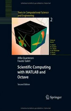
Scientific Computing with MATLAB and Octave PDF
Preview Scientific Computing with MATLAB and Octave
Alfio Quarteroni Fausto Saleri Scientific Computing with MATLAB and Octave Second Edition With108Figuresand12Tables ABC AlfioQuarteroni FaustoSaleri EcolePolytechniqueFédérale MOX-PolitecnicodiMilano deLausanne PiazzaLeonardodaVinci32 CMCS-ModelingandScientificComputing 20133Milano,Italy 1015Lausanne,Switzerland E-mail:fausto.saleri@polimi.it and MOX-PolitecnicodiMilano PiazzaLeonardodaVinci32 20133Milano,Italy E-mail:alfio.quarteroni@epfl.ch CoverfigurebyMarzioSala TitleoftheItalianoriginaledition:IntroduzionealCalcoloScientifico,Springer-VerlagItalia,Milano,2006, ISBN88-470-0480-2 LibraryofCongressControlNumber:2006928277 MathematicsSubjectClassification:65-01,68U01,68N15 ISBN-10 3-540-32612-XSpringerBerlinHeidelbergNewYork ISBN-13 978-3-540-32612-0SpringerBerlinHeidelbergNewYork ISBN-10 3-540-44363-01stEdition SpringerBerlinHeidelbergNewYork Thisworkissubjecttocopyright.Allrightsarereserved,whetherthewholeorpartofthematerialis concerned,specificallytherightsoftranslation,reprinting,reuseofillustrations,recitation,broadcasting, reproductiononmicrofilmorinanyotherway,andstorageindatabanks.Duplicationofthispublication orpartsthereofispermittedonlyundertheprovisionsoftheGermanCopyrightLawofSeptember9, 1965,initscurrentversion,andpermissionforusemustalwaysbeobtainedfromSpringer.Violationsare liableforprosecutionundertheGermanCopyrightLaw. SpringerisapartofSpringerScience+BusinessMedia springer.com (cid:1)c Springer-VerlagBerlinHeidelberg2003,2006 PrintedinTheNetherlands Theuseofgeneraldescriptivenames,registerednames,trademarks,etc.inthispublicationdoesnotimply, evenintheabsenceofaspecificstatement,thatsuchnamesareexemptfromtherelevantprotectivelaws andregulationsandthereforefreeforgeneraluse. Typesetting:bytheauthorsandtechbooksusingaSpringerLATEXmacropackage Coverdesign:design&productionGmbH,Heidelberg Printedonacid-freepaper SPIN:11678793 46/techbooks 543210 http://avaxho.me/blogs/ChrisRedfield Preface Preface to the First Edition This textbook is an introduction to Scientific Computing. We will illustrate several numerical methods for the computer solution of cer- tain classes of mathematical problems that cannot be faced by paper and pencil. We will show how to compute the zeros or the integrals of continuous functions, solve linear systems, approximate functions by polynomials and construct accurate approximations for the solution of differential equations. With this aim, in Chapter 1 we will illustrate the rules of the game thatcomputersadoptwhenstoringandoperatingwithrealandcomplex numbers, vectors and matrices. In order to make our presentation concrete and appealing we will (cid:1) adopt the programming environment MATLAB 1 as a faithful com- panion. We will gradually discover its principal commands, statements and constructs. We will show how to execute all the algorithms that we introduce throughout the book. This will enable us to furnish an im- mediate quantitative assessment of their theoretical properties such as stability, accuracy and complexity. We will solve several problems that willberaisedthroughexercisesandexamples,oftenstemmingfromspe- cific applications. Severalgraphicaldeviceswillbeadoptedinordertorendertheread- ingmorepleasant.WewillreportinthemargintheMATLABcommand along side the line where that command is being introduced for the first time. The symbol will be used to indicate the presence of exercises, the symbol to indicate the presence of a MATLAB program, while 1 MATLABisatrademarkofTheMathWorksInc.,24PrimeParkWay,Nat- ick, MA 01760, Tel: 001+508-647-7000, Fax: 001+508-647-7001. VIII Preface the symbol will be used when we want to attract the attention of the reader on a critical or surprising behavior of an algorithm or a pro- cedure.Themathematicalformulaeofspecialrelevanceareputwithina frame. Finally, the symbol indicates the presence of a display panel summarizing concepts and conclusions which have just been reported and drawn. Attheendofeachchapteraspecificsectionisdevotedtomentioning those subjects which have not been addressed and indicate the biblio- graphical referencesforamore comprehensive treatment of the material that we have carried out. Quite often we will refer to the textbook [QSS06] where many issues facedinthisbookaretreatedatadeeperlevel,andwheretheoreticalre- sultsareproven.ForamorethoroughdescriptionofMATLABwerefer to [HH05]. All the programs introduced in this text can be downloaded from the web address mox.polimi.it/qs Nospecialprerequisiteisdemandedofthereader,withtheexception of an elementary course of Calculus. However,inthecourseofthefirstchapter,werecalltheprincipalre- sultsofCalculusandGeometrythatwillbeusedextensivelythroughout this text. The less elementary subjects, those which are not so neces- saryforanintroductoryeducationalpath,arehighlightedbythespecial symbol . We express our thanks to Thanh-Ha Le Thi from Springer-Verlag Heidelberg,andtoFrancescaBonadeiandMarinaForlizzifromSpringer- Italia for their friendly collaboration throughout this project. We grate- fully thank Prof. Eastham of Cardiff University for editing the language ofthewholemanuscriptandstimulatingustoclarifymanypointsofour text. Milano and Lausanne Alfio Quarteroni May 2003 Fausto Saleri Preface to the Second Edition In this second edition we have enriched all the Chapters by intro- ducing several new problems. Moreover, we have added new methods for the numerical solution of linear and nonlinear systems, the eigen- value computation and the solution of initial-value problems. Another relevant improvement is that we also use the Octave programming en- vironment. Octave is a reimplementation of part of MATLAB which Preface IX includesmanynumericalfacilitiesofMATLABandisfreelydistributed under the GNU General Public License. Throughout the book, we shall often make use of the expression “MATLAB command”: in this case, MATLAB should be understood as the language which is the common subset of both programs MAT- LAB and Octave. We have striven to ensure a seamless usage of our codesandprogramsunderbothMATLABandOctave.Inthefewcases where this does not apply, we shall write a short explanation notice at the end of each corresponding section. For this second edition we would like to thank Paola Causin for hav- ingproposedseveralproblems,ChristophePrud´homme,JohnW.Eaton and David Bateman for their help with Octave, and Silvia Quarteroni for the translation of the new sections. Finally, we kindly acknowledge thesupportofthePoseidon projectoftheEcolePolytechnique F´ed´erale de Lausanne. Lausanne and Milano Alfio Quarteroni May 2006 Fausto Saleri Contents 1 What can’t be ignored................................ 1 1.1 Real numbers ...................................... 2 1.1.1 How we represent them ....................... 2 1.1.2 How we operate with floating-point numbers..... 4 1.2 Complex numbers .................................. 6 1.3 Matrices .......................................... 8 1.3.1 Vectors ..................................... 14 1.4 Real functions ..................................... 15 1.4.1 The zeros ................................... 16 1.4.2 Polynomials ................................. 18 1.4.3 Integration and differentiation ................. 21 1.5 To err is not only human ............................ 23 1.5.1 Talking about costs........................... 26 1.6 The MATLAB and Octave environments ............. 28 1.7 The MATLAB language ............................ 29 1.7.1 MATLAB statements ......................... 31 1.7.2 Programming in MATLAB .................... 32 1.7.3 Examples of differences between MATLAB and Octave languages......................... 36 1.8 What we haven’t told you ........................... 37 1.9 Exercises .......................................... 37 2 Nonlinear equations .................................. 39 2.1 The bisection method ............................... 41 2.2 The Newton method ................................ 45 2.2.1 How to terminate Newton’s iterations........... 47 2.2.2 The Newton method for systems of nonlinear equations.................................... 49 2.3 Fixed point iterations ............................... 51 2.3.1 How to terminate fixed point iterations ......... 55 XII Contents 2.4 Acceleration using Aitken method .................... 56 2.5 Algebraic polynomials............................... 60 2.5.1 Ho¨rner’s algorithm ........................... 61 2.5.2 The Newton-H¨orner method ................... 63 2.6 What we haven’t told you ........................... 65 2.7 Exercises .......................................... 67 3 Approximation of functions and data ................. 71 3.1 Interpolation....................................... 74 3.1.1 Lagrangian polynomial interpolation............ 75 3.1.2 Chebyshev interpolation....................... 80 3.1.3 Trigonometric interpolation and FFT ........... 81 3.2 Piecewise linear interpolation ........................ 86 3.3 Approximation by spline functions.................... 88 3.4 The least-squares method............................ 92 3.5 What we haven’t told you ........................... 97 3.6 Exercises .......................................... 98 4 Numerical differentiation and integration ............. 101 4.1 Approximation of function derivatives................. 103 4.2 Numerical integration ............................... 105 4.2.1 Midpoint formula............................. 106 4.2.2 Trapezoidal formula .......................... 108 4.2.3 Simpson formula ............................. 109 4.3 Interpolatory quadratures ........................... 111 4.4 Simpson adaptive formula ........................... 115 4.5 What we haven’t told you ........................... 119 4.6 Exercises .......................................... 120 5 Linear systems........................................ 123 5.1 The LU factorization method ........................ 126 5.2 The pivoting technique.............................. 134 5.3 How accurate is the LU factorization?................. 136 5.4 How to solve a tridiagonal system .................... 140 5.5 Overdetermined systems............................. 141 5.6 What is hidden behind the command (cid:1)............... 143 5.7 Iterative methods................................... 144 5.7.1 How to construct an iterative method........... 146 5.8 Richardson and gradient methods .................... 150 5.9 The conjugate gradient method ...................... 153 5.10 When should an iterative method be stopped? ......... 156 5.11 To wrap-up: direct or iterative? ...................... 159 5.12 What we haven’t told you ........................... 164 5.13 Exercises .......................................... 164 Contents XIII 6 Eigenvalues and eigenvectors ......................... 167 6.1 The power method ................................. 170 6.1.1 Convergence analysis ......................... 173 6.2 Generalization of the power method .................. 174 6.3 How to compute the shift............................ 176 6.4 Computation of all the eigenvalues.................... 179 6.5 What we haven’t told you ........................... 183 6.6 Exercises .......................................... 183 7 Ordinary differential equations ....................... 187 7.1 The Cauchy problem................................ 190 7.2 Euler methods ..................................... 191 7.2.1 Convergence analysis ......................... 194 7.3 The Crank-Nicolson method ......................... 197 7.4 Zero-stability ...................................... 199 7.5 Stability on unbounded intervals ..................... 202 7.5.1 The region of absolute stability ................ 204 7.5.2 Absolute stability controls perturbations ........ 205 7.6 High order methods................................. 212 7.7 The predictor-corrector methods ..................... 216 7.8 Systems of differential equations...................... 219 7.9 Some examples..................................... 225 7.9.1 The spherical pendulum....................... 225 7.9.2 The three-body problem ...................... 228 7.9.3 Some stiff problems........................... 230 7.10 What we haven’t told you ........................... 234 7.11 Exercises .......................................... 234 8 Numerical methods for (initial-)boundary-value problems ............................................. 237 8.1 Approximation of boundary-value problems............ 240 8.1.1 Approximation by finite differences ............. 241 8.1.2 Approximation by finite elements............... 243 8.1.3 Approximation by finite differences of two-dimensional problems ................... 245 8.1.4 Consistency and convergence................... 251 8.2 Finite difference approximation of the heat equation .... 253 8.3 The wave equation ................................. 257 8.3.1 Approximation by finite differences ............. 260 8.4 What we haven’t told you ........................... 263 8.5 Exercises .......................................... 264 XIV Contents 9 Solutions of the exercises ............................. 267 9.1 Chapter 1 ......................................... 267 9.2 Chapter 2 ......................................... 270 9.3 Chapter 3 ......................................... 276 9.4 Chapter 4 ......................................... 280 9.5 Chapter 5 ......................................... 285 9.6 Chapter 6 ......................................... 289 9.7 Chapter 7 ......................................... 293 9.8 Chapter 8 ......................................... 301 References................................................ 307 Index..................................................... 311 Listings 2.1 bisection: bisection method ........................... 43 2.2 newton: Newton method.............................. 48 2.3 newtonsys: Newton method for nonlinear systems......... 50 2.4 aitken: Aitken method................................ 59 2.5 horner: synthetic division algorithm ..................... 62 2.6 newtonhorner: Newton-H¨orner method ................. 64 3.1 cubicspline: interpolating cubic spline ................... 89 4.1 midpointc: composite midpoint quadrature formula ....... 107 4.2 simpsonc: composite Simpson quadrature formula......... 110 4.3 simpadpt: adaptive Simpson formula.................... 118 5.1 lugauss: Gauss factorization ........................... 131 5.2 itermeth: general iterative method...................... 148 6.1 eigpower: power method.............................. 171 6.2 invshift: inverse power method with shift ................ 175 6.3 gershcircles: Gershgorin circles......................... 177 6.4 qrbasic: method of QR iterations ....................... 180 7.1 feuler: forward Euler method .......................... 192 7.2 beuler: backward Euler method ........................ 193 7.3 cranknic: Crank-Nicolson method ...................... 198 7.4 predcor: predictor-corrector method..................... 218 7.5 onestep: one step of forward Euler (eeonestep), one step ofbackwardEuler(eionestep),onestepofCrank-Nicolson (cnonestep) ........................................ 218 7.6 newmark: Newmark method........................... 223 7.7 fvinc: forcing term for the spherical pendulum problem ..... 227 7.8 threebody: forcing term for the simplified three body system 229 8.1 bvp: approximation of a two-point boundary-value problem by the finite difference method ......................... 242 8.2 poissonfd: approximation of the Poisson problem with Dirichlet data by the five-point finite difference method..... 249
The list of books you might like

As Good as Dead

The 5 Second Rule: Transform your Life, Work, and Confidence with Everyday Courage

Believe Me

What Happened to You?
THIS IS THE AMERICAN EARTH
DTIC ADA448671: Religion and the Military: A Growing Ethical Dilemma
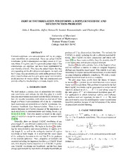
DTIC ADA476425: Zero Autocorrelation Waveforms: A Doppler Statistic and Multifunction Problems
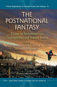
The postnational fantasy: essays on postcolonialism, cosmopolitics and science fiction
Annual Report 2005
byggforskningsrådet
Børns angst for venepunktur

bühnentauglich?

The Psychology of Dexter
Parasitology Today 1993: Vol 9 Index
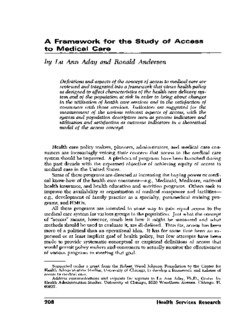
by Lu Ann Aday and Ronald Andersen
Irrigation Works by E S Bellasis

The Brooklyn Paper Volume 29 Issue 22

Depression and your child: a guide for parents and caregivers
Bilgisayar Mühendisliği Programı
Afkondigingsblad van Aruba 2009 no. 12
