Linear Pose Estimation from Points or Lines PDF
Preview Linear Pose Estimation from Points or Lines
IEEETRANSACTIONSONPATTERNANALYSISANDMACHINEINTELLIGENCE, VOL.25, NO.4, APRIL2003 1 Linear Pose Estimation from Points or Lines Adnan Ansar and Kostas Daniilidis, Member, IEEE Abstract—Estimationofcameraposefromanimageofnpointsorlineswithknowncorrespondenceisathoroughlystudiedproblem incomputervision.Mostsolutionsareiterativeanddependonnonlinearoptimizationofsomegeometricconstraint,eitherontheworld coordinatesorontheprojectionstotheimageplane.Forreal-timeapplications,weareinterestedinlinearorclosed-formsolutionsfree ofinitialization.Wepresentageneralframeworkwhichallowsforanovelsetoflinearsolutionstotheposeestimationproblemforboth npointsandnlines.Wethenanalyzethesensitivityofoursolutionstoimagenoiseandshowthatthesensitivityanalysiscanbeused asaconservativepredictoroferrorforouralgorithms.Wepresentanumberofsimulationswhichcompareourresultstotwoother recentlinearalgorithms,aswellastoiterativeapproaches.Weconcludewithtestsonrealimageryinanaugmentedrealitysetup. IndexTerms—Poseestimation,exteriororientation,absoluteorientation,cameralocalization. (cid:1) 1 INTRODUCTION POSEestimationappearsrepeatedlyincomputervisionin approach to ours is taken by Quan and Lan [24]. They many contexts, from visual servoing over 3D input deriveasetofeighthdegreepolynomialconstraintsineven devices to head pose computation. Our primary interest is powers on the depth of each reference point by taking sets in real-time applications for which only a small number of of three inherently quadratic constraints on three variables world objects (lines or points) is available to determine andeliminating twousingSylvesterresultants. Theyapply pose. Augmented reality [2], in which synthetic objects are thismethodtoeachpointinturn.Ouralgorithm,liketheirs, inserted into a real scene, is a prime candidate since a is based on depth recovery, but our approach avoids the potentially restricted workspace demands robust and fast degree increase, couples all n points in a single system of poseestimationfromfewtargets.Themotionofthecamera equations, and solves for all n simultaneously. Recently, is usually unpredictable in such scenarios, so we also Fiore [7] has produced an algorithm for points which require algorithms which are noniterative and require no introduces two scale parameters in the world to camera initialization. transformation and solves for both to obtain the camera In this paper, we propose a novel set of algorithms for coordinates of points. Unlike our algorithm and that of pose estimation from n points or n lines. The solutions are QuanandLan,Fiore’sapproachrequiresatleastsixpoints developed from a general procedure for linearizing quad- unless they are coplanar. We show in Section 4.1, that our ratic systems of a specific type. If a unique solution for the algorithm outperforms both of these linear algorithms in poseproblemexists,thenouralgorithmsareguaranteedto termsofaccuracy.Wealsomention theapproachofTriggs return it. They fail in those cases where there are multiple [27] which uses multiresultants to solve a polynomial discrete solutions. Hence, we can guarantee a solution for system derived from the image of the absolute quadric. n(cid:1)4, provided the world objects do not lie in a critical This method is best suited to four or five points and does configuration [21], [26]. The only similar noniterative not perform as well as direct decomposition of the methods for an arbitrary number of points are those of projection matrix for larger collections of points. Quan and Lan [24] and Fiore [7]. We are aware of no There are many closed form solutions to the three point competing method for lines, but show that our results are problem,suchas[4],[10],whichreturnsolutionswithwell qualitatively acceptable in comparison to an iterative understood multiplicities [15], [22]. Fischler and Bolles [8] algorithm of Kumar and Hanson [16]. extendedtheirsolutiontofourpointsbytakingsubsetsand 1.1 Related Work using consistency checks to eliminate the multiplicity for most point configurations. Horaud et al. [11] developed a Our goal has been to develop fast pose estimation closed form solution on four points, which avoids this algorithmswhichproducestableresultsforasmallnumber reduction to a three point solution. These closed form ofpointorlinecorrespondences.Inthepointcase,asimilar methods can be applied to more points by taking subsets and finding common solutions to several polynomial . A. Ansar is with the Jet Propulsion Laboratory, California Institute of systems, but the results are susceptible to noise and the Technology,4800OakGroveDrive,Pasadena,CA91109. solutions ignore much of the redundancy in the data. E-mail:Adnan.I.Ansar@jpl.nasa.gov. There exist many iterative solutions based on minimiz- . K.DaniilidisiswiththeGRASPLaboratory,UniversityofPennsylvania, 3401WalnutStreet,Suite300C,Philadelphia,PA19104-6228. ingtheerrorinsomenonlineargeometricconstraints,either E-mail:kostas@grasp.cis.upenn.edu. on the image or target. We mention just a few. Nonlinear Manuscript received 19 Dec. 2001; revised 4 Sept. 2002; accepted 10 Sept. optimizationproblemsofthissortarenormallysolvedwith 2002. some variation of gradient descent or Gauss-Newton RecommendedforacceptancebyR.Sharma. methods. Typical of these approaches is the work of Lowe For information on obtaining reprints of this article, please send e-mail to: tpami@computer.org,andreferenceIEEECSLogNumber115596. [19] and of Haralick [5]. There are also approaches which 0162-8828/03/$17.00(cid:1)2003IEEE PublishedbytheIEEEComputerSociety 2 IEEETRANSACTIONSONPATTERNANALYSISANDMACHINEINTELLIGENCE, VOL.25, NO.4, APRIL2003 morecarefullyincorporatethegeometryoftheprobleminto singularvaluesin(cid:1).1IfKerðMÞisone-dimensional,thenxx(cid:1) theupdatestep.Forexample,KumarandHanson[16]have is recovered up to scale. However, the condition (cid:1)¼1 developedanalgorithmbasedonconstraintsonimagelines determines scale and returns the correct solution to (2), using an update step adapted from Horn’s [13] solution of from which we recover the solution to (1) up to a uniform therelativeorientationproblem.Wecomparethisalgorithm sign error. In practice, the physical interpretation of the to our line algorithm in Section 4.1. There are several such problem will determine sign. variations using image line data. Liu et al. [18] use a If the dimension of KerðMÞ is N >1, we attempt to combinationoflineandpointdata.Luetal.[20]combinea isolate the solution to (1) by reimposing the quadratic constraint on the world points, effectively incorporating nature of the original problem. Since xx(cid:1)2KerðMÞ, there depth,withanoptimalupdatestepintheiteration.Weuse exist real numbers f(cid:2)ig such that this as a reference in Section 4, to compare the three linear N point algorithms mentioned. Dementhon and Davis [3] X xx(cid:1)¼ (cid:2)v: ð4Þ i i initialize their iterative scheme by relaxing the camera i¼1 model to scaled orthographic. These iterative approaches Foranyintegersfi;j;k;lgandanypermutationfi0;j0;k0;l0g, typically suffer from slow convergence for bad initializa- tion,convergencetolocalminima,andtherequirementofa observe that xijxkl ¼xi0j0xk0l0. Substituting individual rows from the right-hand side of (4) into relations of this sort largenumberofpointsforstability.Ouralgorithmsrequire noinitialization,canbeusedforasmallnumberofpointsor results, after some algebra, in constraints on the (cid:2)i of the lines, and guarantee a unique solution when one exists. form Anotherapproachistorecovertheworldtoimageplane N projection matrix and extract pose information. This X(cid:2) ðvijvkl(cid:2)vi0j0vk0l0Þþ aa a a a a technique is examined by [1], [9] among many others. This a¼1 ð5Þ projective approach is inherently less stable for pose N N estimation because of the simultaneous solution for the X X 2(cid:2)abðviajvkbl(cid:2)via0j0vkb0l0Þ¼0; calibration parameters. It also requires a large data set for a¼1b¼aþ1 accuracy. We compare this approach to oursin Section4.1. where we use the notation (cid:2)ab ¼(cid:2)a(cid:2)b for integers a and b, andviaj referstotherowofva correspondingtothevariable 2 POSE ESTIMATION ALGORITHM xij in xx(cid:1). We again have the obvious relation (cid:2)ab ¼(cid:2)ba. It follows that equations of the form (5) are linear and Throughoutthispaper,weassumeacalibratedcameraand a perspective projection model. If a point has coordinates homogeneous in the NðN2þ1Þ variables f(cid:2)abg. These can be ðx;y;zÞT in the coordinate frame of the camera, its written in the form K(cid:2)(cid:2)(cid:1)¼0, where K is the matrix of projection onto the image plane is ðx=z;y=z;1ÞT. coefficientsfrom(5)and(cid:2)(cid:2)(cid:1)isthevectorformedbytheterms f(cid:2)abg. We again solve this system by SVD, where 2.1 Mathematical Framework K¼UU~(cid:1)(cid:1)~VV~T.ObservethatKerðKÞmustbeone-dimensional We begin with a general mathematical treatment from since two independent solutions would allow us to derive which we will derive both our point and line algorithms. twosolutionsto (1),contradicting ouroriginal assumption. Consider a system of m quadratic equations in n variables Havingrecovered(cid:2)(cid:2)(cid:1)uptoscale,werecoverthecorrectscale xi of the form by imposing the condition implied by the last row of (4), bi ¼Xn Xn aijkxixj ði¼1...mÞ; ð1Þ vspLieicsiftichaelllyastthraotwp(cid:2)1ovfL1vþi.(cid:2)H2avvL2inþg..s.o:lvþed(cid:2)NfvorLN(cid:2)(cid:2)(cid:1)¼, h(cid:1)e¼nc1e,wxx(cid:1)h, ewree j¼1 k¼j obtain xi as (cid:4) ffixffiffiii, where the choice of sign for x1 wheretheright-handsideof(1)ishomogeneousinfxig.We determines the sign of xi by sgnðxiÞ¼sgnðx1Þsgnðx1iÞ. Before presenting our pose estimation algorithms, we presentalinearizationtechniquetosolvethissysteminthe special case where the solution is a single point in IRn. Let briefly present a more formal treatment of our approach. LetHQðIRnÞand HLðIRnÞbe the set of quadratic and linear xij ¼xixj and (cid:1)¼1. We rewrite (1) as equations on IRn, respectively, which are homogeneous in Xn Xn the variables. Our approach was to linearize the quadratic a x (cid:2)b(cid:1)¼0 ði¼1...mÞ: ð2Þ ijk ij i system in (1) to the linear one in (2) by applying the map j¼1 k¼j f :HQðIRnÞ!HLðIRnn~Þ defined by fðtitjÞ¼tij; fð1Þ¼(cid:1), Since xij ¼xji, this is a homogeneous linear system in the where nn~¼nðn2þ1Þþ1. This increases the dimension of the nðn2þ1Þþ1variablesf(cid:1);xijj1(cid:3)i(cid:3)j(cid:3)ng.Suchasystemcan solution space to N (cid:1)1 by artificially disambiguating be solved by singular value decomposition. We first write related quadratic terms. Let V0 ¼KerðMÞ as above. We the system as think of V0 as an N-dimensional affine variety in IRnn~. V0 assumes an especially simple form since it is a vector Mxx(cid:1)¼0; ð3Þ subspace of IRnn~. To recover the original solution to (1), we where xx(cid:1)¼ðx11 x12...xnn (cid:1)ÞT and M is the matrix of impose additional constraints of the form xijxkl ¼xi0j0xk0l0 coefficients of the system (2). Then, xx(cid:1)2KerðMÞ. If M¼U(cid:1)VT is the SVD, then KerðMÞ¼spanðfvigÞ where the1.seKteorðfÞvreecfetorsrstomtahpepkeedrnteolzoerrno.ulSlsppaancðeÞoreffaerlsinteoarthtreanspsfaonrmoaftiaonse,ti.eo.f, fvig are the columns of V corresponding to the zero vectors,thesetofalllinearcombinationsofthesevectors. ANSARANDDANIILIDIS: LINEARPOSEESTIMATIONFROMPOINTSORLINES 3 forfi0;j0;k0;l0gapermutationoffi;j;k;lg.Lete1beonesuch equation, and let Varðe1Þ be the algebraic variety in IRnn~ defined by it. Then, V1 ¼V0\Varðe1Þ is a subvariety of V0 definedbytheei andthesystem(2).SinceVarðe1Þisnotin any linear subspace of Rnn~, it follows that V1 is a proper subvariety of V0. Given a sequence of such constraints feig with ei independent of fejjj<ig, we obtain a nested sequence of varieties V0 (cid:5)V1 (cid:5)V2... of decreasing dimen- sion. Since we have more quadratic constraints than the dimension of V0, we eventually arrive at the desired solution. Observe that this procedure is entirely generic and does not depend on the coefficients of the original Fig.1.Thebasicgeometricconstraintusedinnpointalgorithmrelates system (1). It follows that an abstract description of the thedistancebetweenpointsintheworlddijandthescalefactorstiand subspace S ¼VarðfeigÞ(cid:6)IRnn~, which we do not yet have, tj associatedwiththeprojectionspi andpj. would allow us to eliminate the second, often more computationally intensive, SVD needed to find KerðKÞ in However, the knowledge of sign implies that we can write our procedure. Note that we are aware of the problems thisas overdimensioning can cause when seeking solutions in a p x ¼sgnðxÞsgnðx Þ ffixffiffiffiffiffixffiffiffiffiffi¼xx y givenparameterspaceinthepresenceofnoise,forexample, ij i jp ii jj i j ij ¼sgnðyÞsgnðy Þ ffiyffiffiffiffiyffiffiffiffiffiffi¼yy : in determining the Essentialmatrix. However, theseeffects i j ii jj i j aredeterminedbythegeometryoftheunderlyingspace.In Thisexplicitdecompositionimpliesthatxx(cid:1)andyy(cid:1)correspond our case, the genericity of S and the linear nature of V0 to solutions consistent with the original quadratic system contributes to the robustness which we see in Section 4. (1). This contradicts the uniqueness assumption on the We now examine the variety S in more detail. For the solution to the original system. moment, we will ignore the constant (cid:1) since it was introduced only as a computational trick. As seen below, 2.2 Point Algorithm fortheproblemsunderconsideration,wealwaysknowthe We assume that the coordinates of n points are known in signs of fxig, hence, fxijg. We now observe that the only someglobalframe,andthatforeveryreferencepointinthe essential relations of the form xijxkl ¼xi0j0xk0l0 are those world frame, we have a correspondence to a point on the which can be written as image plane. Our approach is to recover the depths of x x ¼x2: ð6Þ points by using the geometric rigidity of the target in the ii jj ij form of the nðn(cid:2)1Þ distances between n points. 2 Since fi0;j0;k0;l0g is a permutation of fi;j;k;lg, we have Let wi and wj be two points with projections pi and pj. trivially that We indicate by dij the distance between wi and wj. Let ti x x x x ¼x x x x : andtj bepositiverealnumberssothatjtipijisthedistance ii jj kk ll i0i0 j0j0 k0k0 l0l0 of the point wi from the optical center of the camera, Now, substituting (6), we obtain similarly for tj. It follows that dij ¼jtipi(cid:2)tjpjj. This is our x2x2 ¼x2 x2 : basicgeometricconstraint(seeFig.1).Letbij ¼d2ij.Then,we ij kl i0j0 k0l0 have Sinceweknowthesignsofallxij,takingthesquarerootsof b ¼ðtp (cid:2)t p ÞTðtp (cid:2)t p Þ both sides of the above equation and applying the correct ij i i j j i i j j ð7Þ signsresultsinthedesiredxijxkl ¼xi0j0xk0l0.Observealsothat, ¼t2ipTipiþt2jpTjpj(cid:2)2titjpTipj: for four integers i;j;k;l, the polynomials xiixjj(cid:2)x2ij and xkkxll(cid:2)x2klhavezerosetswhicharecoincident(orsubsetsof Equation (7) is exactly of the form (1), and we apply the oneanotherineitherdirection)onlyiffi;jg¼fk;lg.Itfollows immediatelythatS ¼\fVarðxiixjj(cid:2)x2ijÞg,andthatthisisa solution described to recover the(cid:2)depth scal(cid:3)ings ti. In this basisforthevariety.Therearenðn(cid:2)1Þsuchpolynomialsinan case, M in (3) has size nðn(cid:2)1Þ(cid:7) nðnþ1Þþ1 , and can be 2 2 2 nðnþ1ÞdimensionalEuclideanspace.WeexpectthenthatSis written as M¼ðM0jM00Þ, where M0 is nðn(cid:2)1Þ(cid:7)nðn(cid:2)1Þ 2 2 2 n-dimensional.Thisisclearifwenoticethatonlythevariables diagonal. M has the explicit form fxiigareindependent.Ifthereisasolutiontothequadratic system(1),itfollowsimmediatelythatthelinearizedversion M¼ ofthissolutionssatisfies(2)andthatitliesinthevarietyS. 0(cid:2)2p12 0 0 ... 0 (cid:4)(cid:4)p11 p22 0 ... ... (cid:2)c12 1 (cid:4) Suppose the physical solution is unique. We have already BB 0 (cid:2)2p13 0 ... 0 (cid:4)(cid:4)p11 0 p33 ... ... (cid:2)c13 CC established that there is no sign ambiguity in fxig or fxijg. B@ ... ... ... ... ... (cid:4)(cid:4) ... ... ... ... ... ... CA: Supposethatouralgorithmproducestwosolutionsxx(cid:1)andyy(cid:1). (cid:4) 0 0 0 ... (cid:2)2pn(cid:2)1;n(cid:4)0 ... ... pn(cid:2)1;n(cid:2)1 pnn (cid:2)cn(cid:2)1;n BothofthesemustthenbeinKerðMÞandinS.However,if ð8Þ they are in S, it follows that for x2ij ¼xiixjj and y2ij ¼yiiyjj. 4 IEEETRANSACTIONSONPATTERNANALYSISANDMACHINEINTELLIGENCE, VOL.25, NO.4, APRIL2003 It follows that KerðMÞ is nðnþ1Þþ1(cid:2)nðn(cid:2)1Þ¼nþ1 2 2 dimensional. Hence, we must compute K and find its kernel. K will have ðnþ1Þðnþ2Þ rows and there are Oðn3Þ 2 equationsoftheform(5).Weuseonlythen2ðn(cid:2)1Þconstraints 2 derived from expressions of the form tiitjk ¼tijtik. The choice of sign for ftig is clear, since these are all positive depth scalings. Given these scale factors, we have thecoordinatesofworldpointsintheframeofthecamera. Now, the recovery of camera rotation and translation simply amounts to solving the absolute orientation pro- blem. We translate the two clouds of points, in the camera andworldframes,totheirrespectivecentroidsandrecover the optimal rotation using unit quaternions [12] or SVD of the cross-covariance matrix [14]. Given the rotation, translation between the two centroids is immediately Fig. 2. Geometric constraint used in n line algorithm. The plane Pi recovered. determinedbythelineli andtheopticalcenterisspannedbyf(cid:3)(cid:3)(cid:1)i;(cid:4)(cid:4)(cid:1)ig. We summarize the point algorithm: Thus, wi¼Rivi can be written as a linear combination of these two vectors. 1. Establish quadratic equations in point depths with coefficients dependingon image measurementsand Rvi ¼ðRvTi(cid:3)(cid:3)(cid:1)iÞ(cid:3)(cid:3)(cid:1)iþðRvTi(cid:4)(cid:4)(cid:1)iÞ(cid:4)(cid:4)(cid:1)i. From this, we develop a set distances between 3D points using (7). ofquadraticequationsintheentriesofRtoobtainasystem 2. Rewrite quadratic depth terms titj as tij. oftheform(1)anddirectlyrecovertherotationmatrix.Let 3. Solve resulting linear system in (8). 4. Express real solution as linear combination of basis Ki;j ¼vTivj. We have the equation vectors of KerðMÞ with unknown f(cid:2)ag as in (4). K ¼½ðRvT(cid:3)(cid:3)(cid:1)Þ(cid:3)(cid:3)(cid:1) þðRvT(cid:4)(cid:4)(cid:1)Þ(cid:4)(cid:4)(cid:1)(cid:8)T½ðRvT(cid:3)(cid:3)(cid:1) Þ(cid:3)(cid:3)(cid:1) þðRvT(cid:4)(cid:4)(cid:1)Þ(cid:4)(cid:4)(cid:1)(cid:8): 5. Use relations of the form xijxkl ¼xi0j0xk0l0 for i;j i i i i i i j j j j j j fi0;j0;k0;l0g a permutation of fi;j;k;lg to establish ð9Þ quadratic relations between f(cid:2)ag. For i6¼j, we obtain three additional equations from 6. Rewrite as linear relations in terms f(cid:2)abg and solve using (5). Rv (cid:7)Rv ¼½ðRvT(cid:3)(cid:3)(cid:1)Þ(cid:3)(cid:3)(cid:1) þðRvT(cid:4)(cid:4)(cid:1)Þ(cid:4)(cid:4)(cid:1)(cid:8) i j i i i i i i 7. Recover depths ftig using f(cid:2)ag. (cid:7)½ðRvT(cid:3)(cid:3)(cid:1) Þ(cid:3)(cid:3)(cid:1) þðRvT(cid:4)(cid:4)(cid:1)Þ(cid:4)(cid:4)(cid:1)(cid:8): ð10Þ 8. Solve absolute orientation problem to recover pose. j j j j j j Observethat(9)and(10)donotenforcetherequirement 2.3 Line Algorithm that R2SOð3Þ. We accomplish this using the 12 quadratic Unlike the point case, direct recovery of line parameters constraints derived from does not appear feasible since the number of linearized variables (derived, for example, from Plu¨cker coordinates) RTR¼RRT ¼I: ð11Þ grows too fast in comparison to the number of available constraints. Instead, we show how to directly recover the Note that, in general, there are only six independent rotation and translation. constraints in (11), but by employing our linearization Let fli ¼ðvi;piÞg be a collection of 3D lines such that in procedure,weintroducemorerelationsonthe45linearized the world coordinate frame fvig are normalized vectors terms frij ¼rirjg, where frig are the nine entries in R. givingthedirectionsofthelinesandfpigarepointsonthe Using(9),(10),and(11),weobtainnð2n(cid:2)1Þþ12equations lines. It follows that, in parametric form, points on li are of the form (1) in the 46 variables f(cid:1); rijg. For n(cid:1)5, we given by tiviþpi for the real parameter ti. If ðR;TÞ2 obtain a solution for R directly from the SVD of the SEð3Þ¼SOð3Þ(cid:7)IR3 is the transformation relating the corresponding M from (3). For n¼4, the additional step world and camera frames, then the corresponding repre- involving the SVD of K is required. Observe that the sign sentationsofthelinesinthecameraframearefli ¼ðwi;qiÞg convention is also determined. Since R2SOð3Þ, we need where wi ¼Rvi and qi ¼RpiþT. Let Pi be the plane only choose the global sign so that detðRÞ¼1. defined by the optical center of the camera and the line li. Havingrecoveredtherotation,wedescribehowtorecover Let the corresponding lines in the image plane of the the translation. Given the point qi on the line li in camera camera be fsi ¼ð(cid:3)(cid:3)(cid:1)i;ciÞg, where (cid:3)(cid:3)(cid:1)i and ci are of the forms coordinates,weprojecttoapointki ¼ðqi;x=qi;z;qi;y=qi;z;1Þon ð(cid:3)i;x;(cid:3)i;y;0ÞT andðci;x;ci;y;1ÞT,respectively,with(cid:3)(cid:3)(cid:1)i normal- the image plane. Since this point is on the line si, we have, ized. Consider the point di on si which is closest to the usingthenotationofthissection, origin of the image plane. Then, d ¼c (cid:2)ðcT(cid:3)(cid:3)(cid:1)Þ(cid:3)(cid:3)(cid:1). Let i i i i i (cid:4)(cid:4)(cid:1)i ¼jjddiijj. It follows that (cid:4)(cid:4)(cid:1)iT(cid:3)(cid:3)(cid:1)i ¼0 so that f(cid:3)(cid:3)(cid:1)i;(cid:4)(cid:4)(cid:1)ig is an qi;zðkTi(cid:4)(cid:4)(cid:1)iÞ(cid:4)(cid:4)(cid:1)i ¼qi;zdi: orthonormalframespanningtheplanePi (seeFig.2).Since Substituting q ¼Rp þT for each line, we obtain two i i wi lies entirely in the plane Pi, we can write it as linear equations in the entries of T. A solution can be wi ¼ðwTi(cid:3)(cid:3)(cid:1)iÞ(cid:3)(cid:3)(cid:1)iþðwTi(cid:4)(cid:4)(cid:1)iÞ(cid:4)(cid:4)(cid:1)i.Substitutingwi ¼Rvi,weobtain obtained by directly applying SVD. ANSARANDDANIILIDIS: LINEARPOSEESTIMATIONFROMPOINTSORLINES 5 MyMx ¼(cid:2)MyM ðxþx Þ: ð14Þ We summarize the line algorithm: e e e In the case of five or more lines, recall that M has full 1. Use invariance of inner products (9), expression of cross product in two independent forms (10), and column rank. It follows that MyMxx~e ¼xx~e. Using this fact, the triangle inequality and the properties of the Frobenius membershipofRinSOð3Þ(11)toestablishquadratic equations in entries of R, the rotation matrix norm, we obtain between world an image coordinate frames. jx j(cid:3)jMyj jM j ðjxjþjx jÞ: 2. Rewritequadratictermsrirj fromentriesofRasrij. e F e F e 3. Solve resulting linear system. At this point, we can choose to ignore the quadratic error 4. For four lines, proceed as with points for multi- term, or we can state, based on observation of a given dimensional kernel. physicalsituationandcamerasetup,thatjxx~ej(cid:3)(cid:5)jxx~j,where 5. For five or more lines, first linear step is sufficient. (cid:5)(cid:3)1foranyreasonablesituationandnoiselevel.Itfollows 6. Using known rotation, write overdetermined linear that system in entries of translation using projection equations and solve using SVD. jxej(cid:3)(cid:2)jMyjFjMejFjxj ð15Þ with 1(cid:3)(cid:2)(cid:3)2, where the experimental evaluation below 3 SENSITIVITY ANALYSIS indicates that the upper limit is a highly conservative Wenowanalyzethesensitivityofthelinearsystemandits estimate.Inaddition,forthelinecasexconsistsofproducts intersection with the variety described above to image of terms from rotation matrices, all of which are bounded noise. Consider the linear system of the form (3). above by one. Thus, we can restate (15) as p ffiffiffiffiffi Mxx(cid:1)¼0: ð12Þ jx j(cid:3) 46(cid:9)(cid:2)jMyj jM j : e F e F Recall that the entries of M are polynomials in the image measurements.Inthepresenceofnoise,thetruecoefficient 3.2 Sensitivity for Points matrix for this system is MM~ ¼MþMe, for some error The point case becomes more complicated by the fact that matrix Me, and the true physical solution to the pose Misrankdeficientandhasamultidimensionalkernel.We problem is xx~¼xþxe, for some error vector xe. In our beginbywritingtheerrortermasxe ¼xpþxn,wherexp 2 notation, fMM~;xx~g represents the true physical system, and K¼KerðMÞ and xn is orthogonal to K. Then, fM;xgrepresentsthesystemperturbedbyimagenoise.We proceed by using standard techniques from matrix pertur- MyMxe ¼MyMðxpþxnÞ¼MyMðxnÞ¼xn; bation theory [25]. and (15) becomes Ifweassumeknowledgeofthenoiseinimagemeasure- ments, we can estimate Me. In particular, we can bound jx j(cid:3)(cid:2)jMyj jM j jxj: ð16Þ jMej for some appropriate matrix norm. For the line case, n F e F these are complicated polynomial expressions, but bounds In other words, we only have an estimate of the error in a can be computed experimentally. In the point case, the direction normal to the kernel of M. Nothing more can be polynomials are simple products and sums of products of obtainedfromthelinearsystem.Wemustnowusethefact image measurement errors. Our concern is not with the that both the perturbed solution x and the correct solution computation of bounds on Me since these depend on a x¼xþxe lie on the variety defined by the relations in (6). clearly defined way on image measurements, but with the Each of the equations of the form xiixjj ¼x2ij defines a nature of xx~e, the error in the recovered solution. We make differentiable manifold in RN, but their intersection does no further mention of the computation of jMej in this not.Thislackofregularitymeanswecannotusedifferential section. properties in a straightforward manner. We first consider the simpler case of five or more lines Instead,webeginbyexaminingthekernelmoreclosely. and then apply a more elaborate analysis to the point RecallthatKisnþ1-dimensionalfornpoints.Ifxiswritten algorithm. We omit the four line case in this treatment. In as the following, we will use j(cid:9)j to indicate the Frobenius F xx(cid:1)¼ðx ...x x ...x ...x x ...x (cid:1)ÞT; norm of a matrix, and j(cid:9)j to indicate the 2-norm of vectors 12 1n 23 2n ðn(cid:2)1Þn 11 nn or matrices, as appropriate. thenusingthenotationofSection2.2withxsreplacingtsto maintain consistency with this section, we write down an 3.1 Sensitivity for Lines explicit basis for K. Let w¼ð1111 ...1ÞT and Using the notation developed above, we write (cid:5)(cid:6) (cid:6) (cid:6) (cid:6) (cid:6) (cid:6) (cid:6) (cid:6)T MM~xx~¼0 vi ¼ p12 ...p1n p23 ...p2n ... pðn(cid:2)1ÞðnÞ p11 ...pnn 0 ; 12 1n 23 2n ðn(cid:2)1Þn 11 nn ðMþM Þðxþx Þ¼0 ð13Þ e e MxþMx ¼(cid:2)M ðxþx Þ: where e e e 8 First, observe that Mxx~¼0.2 We multiply both sides of (13) <12 if k6¼landðk¼iorl¼iÞ by the pseudoinverve of M to obtain (cid:6)kl ¼ 1 if l¼k¼i :0 otherwise: 2. Strictly speaking, Mxx~is not zero. However, in practice, jMxx~j<<1, sincexx~istheclosestsolution(e.g.,viaSVD)tothesystemdefinedbyM. Then, fviji¼1::ng[w is the required basis. The fact that ThisdoesnotdependonthemagnitudeoftheerrorinM. Mvi ¼Mw¼0 for the form of M in (8) is a simple 6 IEEETRANSACTIONSONPATTERNANALYSISANDMACHINEINTELLIGENCE, VOL.25, NO.4, APRIL2003 f a b þf b b (cid:2)f b b calculation. Linear independence is easily established by xx^ ¼ ij jk ik ik ij jk jk ij ik; ð21Þ ii a a b þa b b inspecting the last nþ1 entries in each vector. Note that ij jk ik ik ij jk thisisnotanorthogonalbasis,butwedonotrequirethisfor where our purposes. p p PniS¼i1ncciveiþxpdwliefsorirnealthneumkbeerrnselfcio;fdgM. O,bswereveh,ahvoewexvpe¼r, aij ¼xjj(cid:2)xijpiiji bij ¼xii(cid:2)xijpjijj: thattheonlybasisvectorwhichcontributesacomponentto The other terms are obtained by transposing the indices (cid:1)isw.Since(cid:1)¼1isknownexactly,thereisnoerrorinthis appropriately. direction.Itfollowsthatd¼0.Analternativeinterpretation For eachi,we computexx^ii usingallcombinations ofj;k ofthisfactisthatthe(cid:1)variablecanbeeliminatedfromthe withj6¼i6¼kandforaboundonthefsobtainedfromxn. We need only consider the smallest of these since all outset if we do not require that the linear equation in the firststepofouralgorithmbehomogeneous.Theresultisan relations must be satisfied. Combining the terms xx^ii, bounded as above, and using (17), we obtain a bound on expression of the sort jxpj of the same order as jxnj. It follows that we have ðMþM Þðxþx Þ¼ww(cid:1) )Mx ¼(cid:2)M ðxþx Þ; bounded jxej. e e e e e We mention that the linear approximation above is not since Mx¼ww(cid:1) and where the equations are over one fewer necessary. If we choose to include the terms which are variable. From this point, we would proceed as above. quadratic in the errors, we obtain a quadric from (18) in We write the ij component of xp as xx^ij and the ij txx^hiii;sxx^qjju;xx^aidjriincswteaitdhothfeappllaannee dasefiinne(d19b).yT(h1e7)initseraseccotinoinc ionf componentofxnasxx(cid:2)ij,andfocusonthethreevectorobtained xx^ii;xx^jjinsteadofalineasin(20).Wethenproceedasabove, byprojectionofxpontothexii;xjj; andxijdirections.Wesee but with three conics instead of three lines. We do not attempt to write down a closed form expression for this frominspectionofthebasisvectorsthat,foranyi;j,onlyvi;vj approach. contribute to ðxx^ii;xx^jj;xx^ijÞ. This can then be rewritten as 3D Errors: Note that the above procedure can be adapted (cid:2) (cid:3) withlittlemodificationtohandlethecaseoferrorsinthe3D pciii;pcjjj;c2iþpicjj bysubstitutingtheexplicitformoffvig.Wenow coordinatesoffiducials. Thekeypointisthattheerrorin(cid:1) obtainasimplerelationshipbetweenxx^ii;xx^jj;xx^ij,namely, cannolongerbeassumedtobezero.Hence,theright-hand side of (17) will contain a term depending on estimated (cid:2)2pijxx^ijþpiixx^iiþpjjxx^jj ¼0: ð17Þ errorinthedistancesbetweenworldpoints.Consequently, oneofthetwoerrorplanesintersectedaboveisnotalinear Ifxþxe isthesolutiontotheunperturbedsystemMþMe, subspace of Rn, but rather an affine space, whose distance it must satisfy xiixjj ¼x2ij for all i;j. If we substitute fromtheoriginisafunctionoftheestimatederrorinworld xe ¼xpþxn, we obtain coordinates. ðx þxx^ þxx(cid:2) Þðx þxx^ þxx(cid:2) Þ¼ðx þxx^ þxx(cid:2) Þ2: ð18Þ ii ii ii jj jj jj ij ij ij 4 RESULTS Notethatxx(cid:2)ii;xx(cid:2)jj;xx(cid:2)ij areboundedby(16).Wenowcombine We conduct a number of experiments, both simulated and (17) and (18) and try to impose bounds on xx^ii;xx^jj;xx^ij. We real,totestouralgorithms(hereafterreferredtoasNPLand mentioninpassingthat,althoughxpisorthogonaltoxn,we NLLfornpointlinearandnlinelinear,respectively)under can make no such statement about the vectors ðxx^ii;xx^jj;xx^kkÞ image noise. We compare to the following algorithms: and ðxx(cid:2)ii;xx(cid:2)jj;xx(cid:2)kkÞ. For points: As a first approximation, we ignore all quadratic terms . PM: Direct recovery and decomposition of the full in error in (18), which then becomes projection matrix from six or more points by SVD x xx^ þx xx^ (cid:2)2x xx^ (cid:10)2x xx(cid:2) (cid:2)ðx xx(cid:2) þx xx(cid:2) Þ: ð19Þ methods [6]. We use a triangle (4) to indicate this ii jj jj ii ij ij ij ij ii jj jj ii algorithm on all graphs. We rewrite the right-hand side of (19) as fij. Since fij . F: The n point linear algorithm of Fiore [7]. We depends only on terms in x and xn, we can bound it signify this by a square (ut). explicitly. Solving for xx^ij and substituting into (17), we . QL: The n point linear algorithm of Quan and Lan obtain a line in xx^ii;xx^jj given by [24]. We signify this by a diamond ((cid:11)). . LHM: The iterative algorithm of Lu et al. [20] (cid:5)x (cid:2)x pii(cid:6)xx^ þ(cid:5)xx~ (cid:2)x pjj(cid:6)xx^ ¼f : ð20Þ initialized at ground truth. We signify this by a jj ijp ii ii ijp jj ij circle ((cid:12)) and include it primarily as a reference to ij ii compare the absolute performance of the linear If we take any k with i6¼k6¼j, we obtain two more algorithms. We expect it to achieve the best equations of the form performance. ðx (cid:2)x piiÞxx^ þðx (cid:2)x pkkÞxx^ ¼f For lines: kk ikp ii ii ik p kk ik ik ii p p . KH: The iterative algorithm of Kumar and Hanson ðxkk(cid:2)xjkpjjÞxx^jjþðxjj(cid:2)xjkpkkÞxx^kk ¼fjk: referred to as R_and_T in [16]. We initialize KH at jk jj the ground truth translation and rotation (KHRT However, these are all linear in xx^ii;xx^jj;xx^kk, and we solve signified by 4) and at ground truth translation and them simultaneously to obtain identity rotation (KHT signified by ut). ANSARANDDANIILIDIS: LINEARPOSEESTIMATIONFROMPOINTSORLINES 7 Fig.3.(PointSimulation1)Rotation,Translation,andReprojectionerrorsforsixpointsversusnoiselevel.Weplotresultsforthefivealgorithms, NPL,PM,F,QL,andLHM.NotethatNPLoutperformsallbuttheiterativeLHMwithgroundtruthinitialization. 4.1 Simulation directions. We also only admit noise between (cid:2)3(cid:7) and 3(cid:7). All simulations are performed in MATLAB. We assume In the line case, we again report pixel noise and propagate calibrated virtual cameras with effective focal length to noise in the line parameters following [28]. Unless (diagonal terms in calibration matrix) 1;500 in the point indicated, all plots represent mean values over 400 trials. case and 600 in the line case. We report errors in terms of Point Simulation 1 (Dependence on noise level). We relativerotationerrorandrelativetranslationerror.Forthe vary noise from (cid:7)¼0:5 to 4. For each noise level, we pointcase,wealsoshowRMSreprojectionerror.Eachpose generate400random poses.Foreach pose,we generatesix ðR;TÞiswrittenasðqq(cid:1);TÞ,whereqq(cid:1)isaunitquaternion.For points at random with distances between 0 and 200 from recovered values ðqq(cid:1)r;TrÞ, the relative translation error is the camera. We restrict translations to jTj<100. In Fig. 3, computed as 2 jT(cid:2)Trj and the relative rotation error as the observe that NPL outperforms PM, F, and QL for all noise jTjþjTrj absolute error in the unit quaternion, jqq(cid:1)(cid:2)qq(cid:1)rj. For n points levels. with real projections fpg and recovered projections fp g, PointSimulation2(Dependenceonnumberofpoints). i ir the RMS reprojection error is We demonstrate that all five algorithms perform better as thenumberofpointsusedforposeestimationisincreased. vffiffiffiffiffiffiffiffiffiffiffiffiffiffiffiffiffiffiffiffiffiffiffiffiffiffiffiffiffiffiffiffiffiffiffiffiffiffiffiffi uut Xn jp (cid:2)p j2!=n: Points and poses are generated exactly as in Point i ir Simulation 1, but the number of points is varied from five i¼1 to 11. We add 1:5(cid:7)1:5 pixel Gaussian noise to all images. Notethatreprojectionerrorsarecomputedwithadifferent Note, in Fig. 4, that NPL outperforms the other linear set of random points than those used to estimate pose. In algorithms, but that the performance difference is greatest the case of PM, the reprojection is performed with the for fewer points, which is our primary concern as recovered projection matrix rather than by applying the mentioned in the introduction. Note that we do not plot world to camera transformation. Hence, the reprojection results for PM or F for five points since these algorithms error can be smaller than for some linear methods, but require at least six points. never in comparison to NPL. Noise levels in image Point Simulation 3 (Dependence on effective field of measurements are reported in terms of the standard view). We generate poses as in Point Simulation 1. deviation of a zero mean Gaussian. For the point case, However, we now constrain the six points to lie on six of when we add Gaussian noise with standard deviation (cid:7) to the vertices of a 10(cid:7)10(cid:7)10 cube with arbitrary orienta- image coordinates, we do so independently in the x and y tion, but centered on the optical axis of the camera. Once Fig.4.(PointSimulation2)Rotation,Translation,andReprojectionerrorsversusnumberofpointsusedforposeestimationwith1.5(cid:7)1.5pixel Gaussiannoise.WeplotresultsforthefivealgorithmsNPL,PM,F,QL,andLHM.WeseethatNPLoutperformsallbuttheiterativeLHMwith groundtruthinitializationforallnumbersofpointsconsidered.Thedifferenceislargestforasmallnumberofpoints. 8 IEEETRANSACTIONSONPATTERNANALYSISANDMACHINEINTELLIGENCE, VOL.25, NO.4, APRIL2003 Fig.5.(PointSimulation3)Rotation,Translation,andReprojectionerrorsforsixpointsversusextentofobjectgivenasdistance/sizewith1.5(cid:7)1.5 pixelGaussiannoise.Weplotresultsforthefivealgorithms,NPL,PM,F,QL,andLHM.WeseethatNPLoutperformsallbuttheiterativeKHwith groundtruthinitializationintheregioninwhichweareinterested. again, we take 31 point configurations for each of the 31 fixed noise of 1:5(cid:7)1:5 pixels. We see in Fig. 7, that the randomposes.Weadd1.5(cid:7)1.5pixelGaussiannoisetoall performance of both algorithms improves with increasing images. Our goal is to evaluate the performance of our numberoflines.NotealsothatKHislesslikelytoconverge algorithm as the object occupies a smaller fraction of the to local minima for larger numbers of lines. The absolute image.ResultsarerecordedinFig.5.NPLoutperformsQL, performance of NLL is again comparable to KH. PM, and F for pose estimation when the object is approximately seven times as far away as its extent. Note 4.1.1 Timings in Simulation that this is our primary region of interest. Wecomparetheruntimesofourproceduretoseveralothers Line Simulation 1 (Dependence on noise level). We using MATLAB implementations of all algorithms on a 1.1 varypixelnoisefrom(cid:7)¼0:5to5andpropagatetonoisein GHzPentiumIIIprocessor.Notethatrealtimeperformance line parameters following [28]. For each noise level, we is not expected for any of the algorithms under MATLAB, generate 400 poses and six line segments for each pose. and our only goal is to provide comparison. The iterative World linesegments arecontained in a20(cid:7)20(cid:7)20 box in algorithms (KH and LHM) were set to terminate after 100 front of the camera and translations are restricted to iterations if convergence had not yet been achieved. All jTj<10. We plot relative rotation and translation errors resultsareaveragedover1,000trialsandforpointsorlines for NLL and KH (see Fig. 6). As expected, the iterative ranging from 6 to 11. The results are recorded in Table 1. algorithm performs better for good initialization (ground The notation used is identical to that above with the truth in the case of KHRT). However, we cannot predict following additions: convergence time. With poor initialization, even at ground truth translation and R¼I for KHT, our linear algorithm . LHMPM: refers to LHM initialized with the output shows better mean performance. This is a result of of PM. convergencetolocalminimainsometrials.Wedemonstrate . LHMT:referstoLHMinitializedatidentityrotation this by plotting not only mean relative rotation and and ground truth translation (analogous to KHT as translation errors, but also the standard deviation of the defined above for lines). relativerotationerror.Weimmediatelyseetheadvantageof . KHNLL: refers to KH initialized with NLL. having no initialization requirement for NLL. We see that in the implementations tested, LHMPM is Line Simulation 2 (Dependence on number of lines). consistentlyfasterthanourpointalgorithm(NPL),withthe WegenerateposesandpointsasinLine Simulation1,but difference increasing with the number of points. However, for the numbers of lines varying from four to 11 and with as indicated in Section 4.2, for the number of points under Fig.6.(LineSimulation1)RotationandTranslationerrorsandStandardDeviationofRotationerrorversusnoiselevelforNLLandKH.Weinitialize KHatgroundtruthRandT(KHRT)toevaluateabsoluteperformanceandatgroundtruthTandR¼I(KHT)todemonstratetheadvantageof requiringnoinitializationinNLL. ANSARANDDANIILIDIS: LINEARPOSEESTIMATIONFROMPOINTSORLINES 9 Fig.7.(LineSimulation2)RotationandTranslationerrorsandStandardDeviationofRotationerrorversusnumberofpointsforNLLandKH.Noise isfixedat1:5(cid:7)1:5pixels.WeinitializeKHatgroundtruthRandT(KHRT)toevaluateabsoluteperformanceandatgroundtruthTandR¼I (KHT)todemonstratetheadvantageofrequiringnoinitializationinNLL. consideration our algorithm runs in realtime under a C for the number of points discussed above and without any implementation on a 600 MHz Pentium III. In addition, attempt to optimize the algorithm. unlikeLHM,weguaranteerecoveryofthesolutionwhenit PointExperiment1.Wedemonstratethatvirtualobjects exists andrequireno initialization.Forthe linecase(NLL), arecorrectlyregisteredintoarealsceneusingNPLforpose our algorithm is faster than KH. Since NLL is less estimation. We obtain the coordinates of the eight marked computationally intensive than NPL, we expect perfor- points in Fig. 8, by magnifying the relevant region and marking by hand with a MATLAB program. We take the mance from a C implementation at video framerate with vertex coordinates of a virtual box and the corners of the this algorithm as well. metal edge in the world frame, transform to the camera 4.2 Real Experiments frame using the three recovered poses, and reproject. The All images were taken with a Sony XC-999 camera and metal edge, which we augment to a full cube, is seven MatroxMeteorIIframegrabber.Thecamerawascalibrated inchesoneachside,andthecameradistancevariesfrom30 using Lenz andTsai’s algorithm [17]. All image processing to40inchesfromthenearestcornerofthecube.Noticethat was done offline using MATLAB. Note that the more the virtual boxes are properly placed and aligned with the computationally intensive point algorithm NPL has been world reference objects for all three poses. PointExperiment2.WerepeatPointExperiment1ona runinreal-time(>30Hz)ona600MHzPentiumIIIusing differentscale.InFig.9,theboxisapproximately18inches theimplementationofSVDfromnumericalrecipesinC[23] on each side, and the camera is approximately eight feet from the nearest corner of the box. We estimate pose from TABLE 1 the eight marked points using NPL. We then take the TimingResults (inSeconds)forAlgorithms UnderMATLAB coordinatesoftwovirtualboxesofidenticalsize,stackedon on a1.1GHzPentium III top of and next to the real one, transform to camera coordinates, and reproject into the image. Note that the virtualboxesareverycloselyalignedwiththerealoneand appear to be the correct size. PointExperiment3.WetestNPLoncoplanarpoints.In Fig. 10, we mark nine points on the calibration grid in the image. The points have a uniform spacing of eight inches. The camera is placed approximately 11 feet from the marked points. We recover the coordinates of the nine points using NPL and compute a best fit plane from the recovered points. The mean distance from the recovered points to the best fit plane is 0.15 inches with a standard deviationof0.07inches.Weseethatouralgorithmdoesnot degenerate for coplanar points. LineExperiment1.Wedemonstratethecorrectregistra- tion of virtual objects into a real scene using NLL. In Fig. 11a, we indicate the seven line segments used to estimate camera pose. In Fig. 11b, we overlay a texture on the faces of the pictured box by transforming the world coordinates of the box vertices to camera coordinates and Results are given for NPL, PM, QL, F, LHMPM (LHM initialized with warping the texture onto the resulting quadrangles via PM), LHMT (LHM initialized with identity rotation and ground truth translation),KHNLL(KHinitializedwithNLL),andKHT(KHinitialized homographies.We alsoplaceavirtual cubeonthe original withidentityrotationandgroundtruthtranslation). box. The cube is aligned with the real box in world 10 IEEETRANSACTIONSONPATTERNANALYSISANDMACHINEINTELLIGENCE, VOL.25, NO.4, APRIL2003 Fig.8.(PointExperiment1).Reprojectionofavirtualboxandthreeedgesofacubeontoreal-worldreferenceobjects.Weestimatecamerapose usingtheeightcircledpointsandNPL. coordinates. Observe that, after transformation to the line are underestimation of error, and points below the camera frame and reprojection, it remains aligned. Finally, line are overestimations. Note that underestimation in we highlight the edges of the table by transforming its some cases is to be expected. First, the linear approxima- world coordinates to camera coordinates and reprojecting tion in (19) will have an effect. Also, (21) has obvious the appropriate line segments. We emphasize that all singularities for certain configurations which we have not virtual objects are constructed in world coordinates and treated separately. Fig. 12a represents (cid:2)¼1 in (16). In inserted into the images only after pose estimation and this case, approximately 4.5 percent of the trials resulted transformation to camera coordinates. in underestimation of errors. Fig. 12b represents (cid:2)¼2. Here, approximately 1 percent of the trials resulted in 4.3 Error prediction underestimation of the error. We show that the sensitivity analysis of Section 3 can be usedtoestimateerrorsintherecovereddepthsforthepoint 5 CONCLUSION algorithm,givensomeideaofthegeometryoftheproblem. Wefocusonthepointalgorithmsincetheresultfortheline Our goal was to develop fast and accurate pose estimation algorithm is a direct application of linear algebra techni- algorithmsforalimitednumbersofpointsorlines.Wehave ques. Since our goal is to show the applicability of the presented a general mathematical procedure from which overall procedure, we do not attempt to estimate Me. we derive a pair of linear algorithms which guarantee the Rather,wewillusethegroundtruthMM~ tofindMe exactly, correctsolutioninthenoiselesscase,provideditisunique. and then calculate xn using this. For each point i, we Wedevelop asensitivityanalysisfor ouralgorithmswhich estimatexp,theerrorinthekerneldirectionusing(21)over also allows for coarse estimation of errors (with under- alljandk.Wethentakethesmallestofthesesinceallmust estimation in very few cases) in pose recovery based on be approximately satisfied. known image errors. Our point algorithm shows perfor- We plot results for various levels of Gaussian noise mance superior to competing linear algorithms and ranging from 0.5 to five pixel standard deviation. For comparable to a recent iterative algorithm. For our line each noise level, we take 200 trials of six points with algorithm,thereisnocompetinglinearapproach.Weshow translation restricted to half the maximum scene depth. resultscomparabletoarobustiterativealgorithmwhenitis We plot in Fig. 12, the ratio of the norm of the real error correctlyinitializedandavoidtheproblemsassociatedwith (computed from ground truth) to the estimated error local minima for such algorithms. from the sensitivity analysis on a semilog scale. The horizontal lines represent a ratio of one. Points above the Fig.10.(PointExperiment3).Werecoverthecoordinatesofthenine Fig. 9. (Point Experiment 2). Reprojection of two virtual boxes of coplanar points marked above using NPL and calculate the mean dimensionsidenticaltoarealbox.Weestimatecameraposeusingthe distancebetweenrecoveredpointsandabestfitplaneas<1%ofthe eightcircledpointsandNPL. sizeofthesquaredefinedbytheninepoints.
Description:The list of books you might like

The Silent Patient

Do Epic Shit

The 48 Laws of Power

The Subtle Art of Not Giving a F*ck

Mast Cell Biology: Contemporary and Emerging Topics

00. Il Trono di Ghiaccio - La Lama dell’Assassina
FHSU Block & Bridle Club Scrapbook: 2005-2006

NASA Technical Reports Server (NTRS) 20050241962: International Heliophysical Year
Экологический практикум. 5(6) класс

Kluftinger: Kriminalroman (Kluftinger-Krimis 10) (German Edition)

Environmental Management of Waste Electrical and Electronic Equipment

Vanity All is Vanity by J J Cranmer

The Missing README

ANSI NEMA CC-1-2009 Electric Power For Substations

A Summary of Lightpipe Radiation Thermometry Research at NIST

NASA Technical Reports Server (NTRS) 20080015510: Utilizing Calibrated GPS Reflected Signals to Estimate Soil Reflectivity and Dielectric Constant: Results from SMEX02

NASA Technical Reports Server (NTRS) 20080014294: Arbitrary Steady-State Solutions with the K-epsilon Model

Die Kaiserliche Marine während der Wirren in China 1900-1901
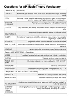
Questions for AP Music Theory Vocabulary

c_paginas INICIAIS_nova.indd

ERIC ED362642: Developments in the Curriculum for the Swedish MSc Programme in Agriculture.
