Efficient Maximum-Likelihood Inference For The Isolation-With-Initial-Migration Model With Potentially Asymmetric Gene Flow PDF
Preview Efficient Maximum-Likelihood Inference For The Isolation-With-Initial-Migration Model With Potentially Asymmetric Gene Flow
Efficient Maximum-Likelihood Inference For The Isolation-With-Initial-Migration Model With Potentially Asymmetric Gene Flow Rui J. Costa and Hilde Wilkinson-Herbots 6 Department of Statistical Science, University College London 1 Gower Street, London WC1E 6BT, UK 0 2 email: rui.costa.11@ucl.ac.uk n a J Abstract 4 1 The isolation-with-migration (IM) model is a common tool to make inferences ] about the presence of gene flow during speciation, using polymorphism data. How- E ever, Becquet and Przeworski (2009) report that the parameter estimates obtained P . by fitting the IM model are very sensitive to the model’s assumptions – including o i the assumption of constant gene flow until the present. This paper is concerned b - with the isolation-with-initial-migration (IIM) model of Wilkinson-Herbots (2012), q which drops precisely this assumption. In the IIM model, one ancestral population [ dividesintotwodescendantsubpopulations,betweenwhichthereisaninitialperiod 1 v ofgeneflowandasubsequentperiodofisolation. Wederiveafastmethodoffitting 4 an extended version of the IIM model, which allows for asymmetric gene flow and 8 6 unequal subpopulation sizes. This is a maximum-likelihood method, applicable to 3 observations on the number of segregating sites between pairs of DNA sequences 0 from a large number of independent loci. In addition to obtaining parameter es- . 1 timates, our method can also be used to distinguish between alternative models 0 6 representing different evolutionary scenarios, by means of likelihood ratio tests. We 1 illustratetheprocedureonpairsofDrosophilasequencesfromapproximately30,000 : v loci. The computing time needed to fit the most complex version of the model to i X this data set is only a couple of minutes. The R code to fit the IIM model can be r found in the supplementary files of this paper. a Keywords: speciation, coalescent, maximum-likelihood, gene flow, isolation 1 1 Introduction The2-demeisolation-with-migration(IM)modelisapopulationgeneticmodelinwhich, at some point in the past, an ancestral population divided into two subpopulations. After the division, these subpopulations exchanged migrants at a constant rate until the present. The IM model has become one of the most popular probabilistic models in use to study genetic diversity under gene flow and population structure. Although applicable to populations within species, many researchers are using it to detect gene flowbetweendivergingpopulationsandtoinvestigatetheroleofgeneflowintheprocess of speciation. A meta-analysis of published research articles that used the IM model in the context of speciation can be found in Pinho and Hey (2010). Several authors have developed computational methods to fit IM models to real DNA data. Some of the most used programs are aimed at data sets consisting of a large number of sequences from a small number of loci. This is the case of MDIV (Nielsen and Wakeley, 2001), IM (Hey and Nielsen, 2004; Hey, 2005), IMa (Hey and Nielsen, 2007) and IMa2 (Hey, 2010), which rely on Bayesian MCMC methods to estimate the model parameters and are computationally very intensive. In the past decade, the availability of whole genome sequences has increased signif- icantly. Very large data sets consisting of thousands of loci, usually from just a few individuals, became available for analysis, and such multilocus data sets are more infor- mative than their single locus counterparts. In fact, as the sample size for a single locus increases, the probability that an extra sequence adds a deep (i.e. informative) branch to the coalescent tree quickly becomes negligible (see, e.g., Hein et al., 2005, p. 28-29). This new type of data set is also much more suitable for likelihood inference: if at each locus the observation consists only of a pair or a triplet of sequences, the coalescent process of these sequences is relatively simple and can more easily be used to derive the likelihood for the locus concerned. Furthermore, if the loci studied are distant from each other, observations at different loci can be considered independent and thus the likelihood of a whole set will consist of the product of the likelihoods for the individual loci. For these reasons, some of the most recent theoretical papers and computer imple- mentations of the IM model are aimed at data sets consisting of a small number of sequences at a large number of loci. Wang and Hey (2010) and Zhu and Yang (2012), for example, developed maximum-likelihood methods based on numerical integration. Computationally less intensive methods of fitting the IM model were studied by Lohse et al. (2011), who used moment generating functions, and Andersen et al. (2014), who 2 resorted to matrix exponentiation and decomposition. Despite all the progress, several authors have recently pointed out some limitations of the IM model. Becquet and Przeworski (2009) report that the parameter estimates obtained by fitting the IM model are highly sensitive to the model’s assumptions – in- cluding the assumption of constant gene flow until the present. Strasburg and Rieseberg (2011) and Sousa et al. (2011) note that the gene flow timing estimates reported in the literature, basedontheIMmodelandobtainedwiththeIMA2 program, haveextremely wide confidence intervals, as the time of gene flow is non-identifiable in the IM model. As a step to overcome these limitations, Wilkinson-Herbots (2012) studied an exten- sion of the IM model, the isolation-with-initial-migration (IIM) model, which is more realisticthantheIMmodelinthecontextofspeciation. Broadlyspeaking,theIIMmodel is an IM model in which gene flow ceased at some point in the past. Explicit formulae for the distribution of the coalescence time of a pair of sequences, and the distribution of the number of nucleotide differences between them, are derived in Wilkinson-Herbots (2012). These analytic results enable a very fast computation of the likelihood of a data set consisting of observations on pairs of sequences at a large number of independent loci. However, for mathematical reasons this work was limited to the case of symmetric migration and equal subpopulation sizes during the migration period. In this paper, we study a more general IIM model which allows for asymmetric gene flow during the migration period. It also allows for unequal subpopulation sizes during gene flow, as well as during the isolation stage. Both this model and other simpler models studied in this paper assume haploid DNA sequences, which accumulate mutations according to the infinite sites assumption (Watterson, 1975). An extension to the Jukes-Cantor model of mutation is feasible but beyond the scope of this paper. We first describe, for different versions of the IIM model, an efficient method to compute the likelihood of a set of observations on the number of different nucleotides between pairs of sequences (also termed the number of pairwise differences). Each pair of sequences comes from a different locus and we assume free recombination between loci and no recombination within loci. Secondly, we illustrate how to use this method to fit the IIM model to real data. The data set of Drosophila sequences from Wang and Hey (2010), containing over 30,000 observations (i.e. loci), is used for this purpose. Finally, we demonstrate, using this data set, how different models, representing different evolutionary scenarios, can be compared using likelihood ratio tests. 3 Figure 1: TheIIMmodel. Theleft-handsidesubpopulationissubpopulation1; theright-hand side subpopulation is subpopulation 2. 2 Theory and methods For the purposes of the present paper, and from a forward-in-time perspective, the isolation-with-migration (IM) model makes the following assumptions: a) until time τ 0 ago(τ > 0),apopulationofDNAsequencesfromasinglelocusfollowedaWright-Fisher 0 haploid model (Fisher, 1930; Wright, 1931); b) at time τ ago, this ancestral population 0 split into two Wright-Fisher subpopulations with constant gene flow between them. If we take an IM model and add the assumption that, at time τ ago (0 < τ < τ ), gene 1 1 0 flow ceased, we get an isolation-with-initial-migration (IIM) model. Figure 1 illustrates the fullest IIM model dealt with in this paper. IntheIIMmodelofFigure1, thepopulationsizesaregiveninsidetheboxes, inunits of DNA sequences. All population sizes are assumed constant and strictly positive. The parameters a, b, c and c indicate the relative size of each population with respect 1 2 to subpopulation 1 during the migration stage. For example, if 2N is the number anc of sequences in the ancestral population, then a = 2N /2N. Between times τ and anc 0 τ ago (two time parameters in units of 2N generations) there is gene flow between the 1 subpopulations: ineachgeneration,afractionm ofsubpopulationiareimmigrantsfrom i subpopulation j (i,j ∈ {1,2} with i (cid:54)= j), i.e. m is the migration rate per generation i from subpopulation i to subpopulation j backward in time. Within each subpopulation, reproduction follows the neutral Wright-Fisher model and, in each generation, restores the subpopulations to their original sizes, i.e. reproduction undoes any decrease or increase in size caused by gene flow (this assumption of constant population size is common and usually reflects restrictions on food and habitat size). 4 Under the IIM model, the genealogy of a sample of two DNA sequences from the presentsubpopulationscanbedescribedbysuccessiveMarkovchains,workingbackward in time. We will define these in the simplest possible way, using the smallest state space necessary for the derivation of the coalescence time distribution. Hence, during the isolation stage (until time τ into the past) and the migration stage (between τ and 1 1 τ ), the process can only be in state 1 – both lineages in subpopulation 1 –, state 2 – 0 both lineages in subpopulation 2 –, state 3 – one lineage in each subpopulation –, or state 4 – in which lineages have coalesced. After τ , the lineages have either coalesced 0 already – state 4 –, or have not – state 0. Only states 1, 2 and 3 can be initial states, according to whether we sample two sequences from subpopulation 1, two sequences from subpopulation 2, or one sequence from each subpopulation. When the genealogical process starts in state i (with i ∈ {1,2,3}), the time until the most recent common ancestor of the two sampled sequences is denoted T(i), whereas S(i) denotes the number of nucleotide differences between them. Iftimeismeasuredinunitsof2N generationsandN islarge,thegenealogicalprocess is well approximated by a succession of three continuous-time Markov chains, one for each stage of the IIM model (Kingman, 1982a,b; Notohara, 1990). We refer to this stochastic process in continuous time as the coalescent under the IIM model. During the isolation stage, the approximation is by a Markov chain defined by the generator matrix (i) (4) (cid:34) (cid:35) Q(i) = (i) −c1i c1i , (1) iso (4) 0 0 with i ∈ {1,2} being the initial state (Kingman, 1982a,b). If 3 is the initial state, the lineages cannot coalesce before τ . During the ancestral stage, the genealogical process 1 is approximated by a Markov chain with generator matrix (0) (4) (0) −1 1 Q = a a . (2) anc (4) 0 0 (Kingman, 1982a,b). In between, during the migration stage, the approximation is by a 5 Markov chain with generator matrix (1) (3) (2) (4) (1) −(1+M1) M1 0 1 Qmig = (3) M22 −(cid:0)M1+2M2(cid:1) M21 0 (3) (2) 0 M2 −(1/b+M2) 1/b (4) 0 0 0 0 (Notohara, 1990). In this matrix, M /2 = 2Nm represents the rate of migration (in i i continuous time) of a single sequence when in subpopulation i. The rates of coalescence for two lineages in subpopulation 1 or 2 are 1 and 1/b respectively. Note that state 3 corresponds to the second row and column, and state 2 to the third row and column. This swap was dictated by mathematical convenience: the matrix Q should be as mig symmetric as possible because this facilitates a proof in the next section. 2.1 Distribution of the time until coalescence under bidirectional gene flow (M > 0, M > 0) 1 2 To find f(i), the density of the coalescence time T(i) of two lineages under the IIM T model, given that the process starts in state i and there is gene flow in both directions, (i) weconsiderseparatelythethreeMarkovchainsmentionedabove. WeletT (i ∈ {1,2}), iso (i) (0) T (i ∈ {1,2,3}) and T denote the times until absorption of the time-homogeneous mig anc (i) Markov chains defined by the generator matrices Q , Q and Q respectively. iso mig anc (i) (i) (0) (i) And we let the corresponding pdf’s (or cdf’s) be denoted by f , f and f (or F , iso mig anc iso (i) (0) (i) F and F ). Then f can be expressed in terms of the distribution functions just mig anc T mentioned: (i) fiso(t) for 0 ≤ t ≤ τ1, (i) (cid:104)1−Fi(sio)(τ1)(cid:105)fm(i)ig(t−τ1) for τ1 < t ≤ τ0, f (t) = (cid:104) (cid:105)(cid:104) (cid:105) (4) T (i) (i) (0) 1−Fiso(τ1) 1−Fmig(τ0−τ1) fanc(t−τ0) for τ0 < t < ∞, 0 otherwise. 6 for i ∈ {1,2}. If 3 is the initial state, (3) fmig(t−τ1) for τ1 < t ≤ τ0, (cid:104) (cid:105) (3) (3) (0) f (t) = 1−F (τ −τ ) f (t−τ ) for τ < t < ∞, (5) T mig 0 1 anc 0 0 0 otherwise. The important conclusion to draw from these considerations is that to find the distribu- tion of the coalescence time under the IIM model, we only need to find the distributions of the absorption times under the simpler processes just defined. A Markov process defined by the matrix Q , and starting in state 0, is simply anc Kingman’s coalescent (Kingman, 1982a,b). For such a process, the distribution of the coalescence time is exponential, with rate equal to the inverse of the relative population size: 1 fa(0n)c(t) = ae−a1t, 0 ≤ t < ∞. (i) A Markov process defined by Q , i ∈ {1,2}, is again Kingman’s coalescent, so iso (i) 1 −1t fiso(t) = c e ci , 0 ≤ t < ∞. i Finally, with respect to the ‘structured’ coalescent process defined by the matrix Q , mig we prove below that, for i ∈ {1,2,3}, 3 f(i) (t) = −(cid:88)V−1V λ e−λjt, (6) mig ij j4 j j=1 where V is the (i,j) entry of the (non-singular) matrix V, whose rows are the left ij eigenvectors of Q . The (i,j) entry of the matrix V−1 is denoted by V−1. The λ mig ij j (j ∈ {1,2,3}) are the absolute values of those eigenvalues of Q which are strictly mig negative (the remaining one is zero). Since the λ are real and strictly positive, the j (i) density function of T is a linear combination of exponential densities. mig Proof of (6): This proof has three parts. Part (i) proves the above result under two assumptions: a) Q has three strictly negative eigenvalues and one zero eigenvalue, all of them mig real; and b) Q is diagonalizable. Part (ii) proves assumption a). Part (iii) proves mig assumption b). To simplify the notation, we denote Q by Q throughout the proof. mig 7 (i) Consider the continuous-time Markov chain defined by the matrix Q. Let P (t), the ij (i,j) entry of the matrix P(t), be the probability that the process is in state j at time t into the past, given that the process starts in state i. P(t) can be calculated by solving the following initial value problem: P(cid:48)(t) = P(t)Q ; P(0) = I , 4 where I is the four by four identity matrix. Under the assumptions that Q is diagonal- 4 izable and that its eigenvalues are real, the solution to this initial value problem is given by: P(t) = P(0)eQt = V−1eBtV , where B denotes the diagonal matrix containing the real eigenvalues β , j ∈ {1,2,3,4}, j of Q, and V is the matrix of left eigenvectors of Q. Note that P (t) is the probability i4 thattheprocesshasreachedcoalescencebytimet, ifitstartedinstatei. Inotherwords, (i) it is the cdf of T : mig P (t) = F(i) (t) = v−1eBtv , i4 mig i. .4 where v−1 is the ith row vector of V−1, and v the 4th column vector of V. Differenti- i. .4 ating, we get the pdf: f(i) (t) = v−1BeBtv mig i. .4 4 (cid:88) = V−1V β eβjt . ij j4 j j=1 Ifwedenotetheeigenvalueequaltozerobyβ ,andtheremainingeigenvaluesarestrictly 4 negative, this pdf can be written as a linear combination of exponential densities: 3 f(i) (t) = −(cid:88)V−1V λ e−λjt , (7) mig ij j4 j j=1 where λ = |β | for j ∈ {1,2,3}. j j 8 (ii) As Q is given by equation (3), its characteristic polynomial, P (β), is of the form Q β ×P (β), where Q(r) is the three by three upper-left submatrix of Q, that is: Q(r) −(1+M ) M 0 1 1 Q(r) = M2/2 −(M1+M2)/2 M1/2 . 0 M −(1/b+M ) 2 2 Thus the eigenvalues of Q are the solutions to β ×P (β) = 0. Consequently, one of Q(r) them is zero (β , say) and the remaining three eigenvalues are also eigenvalues of Q(r). 4 Now consider the similarity transformation (cid:113) −(1+M1) M12M2 0 S = DQ(r)D−1 = (cid:113)M12M2 −(M1+M2)/2 (cid:113)M12M2 , (cid:113) 0 M12M2 −(1/b+M2) (cid:113) M2 0 0 2M1 where D = 0 1 0 . (cid:113) 0 0 M1 2M2 Because S is a symmetric matrix, its eigenvalues are real. Therefore, all the eigenvalues of Q(r) are real (a similarity transformation does not change the eigenvalues). S is also a negative definite matrix, since its first, second and third upper-left determinants are respectively negative, positive, and negative. Hence its eigenvalues are all strictly negative, and so are the eigenvalues of Q(r). Hence Q has one zero eigenvalue (β ) and 4 three real, strictly negative eigenvalues (β ,β and β ). 1 2 3 (iii) Being a symmetric matrix, S has three independent eigenvectors. A similarity transfor- mationpreservesthenumberofindependenteigenvectors, soQ(r) hasthreeindependent eigenvectors as well. We denote by V(r) the matrix whose rows are the left eigenvectors of Q(r). By definition, any left eigenvector v of Q satisfies the system of equations x(Q− j. 9 Iβ ) = 0, where x = [x x x x ]. The first three linear equations of this system are j 1 2 3 4 identical to x(r)(Q(r)−Iβ ) = 0, for j ∈ {1,2,3} and x(r) = [x x x ], which is solved j 1 2 3 byx(r) = v(r). Sothisimpliesthat, forβ ∈ {β ,β ,β }, anyrowvectorxinR4 thathas j. j 1 2 3 (r) v as its first three elements will solve the first three equations of the system, whatever j. the value of x . If x = (V(r) + 1V(r))/β , that vector will be an eigenvector of Q, 4 4 j1 b j3 j because it also solves the fourth equation of the system: −(1+M1)−βj M1 0 1 (cid:104) ——–vj(.r)——– Vj(1r)+βj1bVj(3r) (cid:105) M22 −(M1+2M2) −βj M21 0 0 M −(1 +M )−β 1 2 b 2 j b 0 0 0 −β j (cid:104) (cid:105) = 0 0 0 0 , for β ∈ {β ,β ,β }. For the case of β = β = 0, a row eigenvector is [0 0 0 1]. j 1 2 3 j 4 Collecting these row eigenvectors in a single matrix, we get V. So, (r) (V(r)+1V(r)) —— v —— 11 b 13 1. β1 (r) (V(r)+1V(r)) —— v —— 21 b 23 V = 2. β2 . (r) (V(r)+1V(r)) —— v3. —— 31 β3b 33 0 0 0 1 If the matrix V can be shown to be invertible, then Q is diagonalizable. This will be the case if the system xV = 0 can only be solved by x = [0 0 0 0]. Now since the three by three upper-left submatrix of V, V(r), is full-ranked, x = x = x = 0 is a necessary 1 2 3 condition for xV = 0. But then x = 0, from the last equation of the system. Thus we 4 have shown that Q is diagonalizable. (cid:3) Wearenowinpositiontoupdateequations(4)and(5)withtheresultsjustobtained. 10
The list of books you might like

Believe Me

The 5 Second Rule: Transform your Life, Work, and Confidence with Everyday Courage

Rich Dad Poor Dad

A Thousand Boy Kisses
Appalachian Regional Commission

Did I Mention I Miss You?
DISCOVERY OF SUBULARIA-AQUATICA L IN COLORADO AND THE EXTENSION OF ITS RANGE
Bürgerliches Recht für Betriebswirte: Allgemeiner Teil — Schuldrecht — Sachenrecht
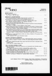
Plant Science 1993: Vol 93 Table of Contents

Right off the Bat by William F Kirk

DTIC ADP023955: Will the Larger Air Force Ever Accept the Space Cadre

Hurst’s the Heart

Cadre d'évaluation et d'analyse de l'enquête PISA pour le développement
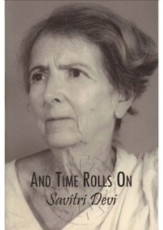
And Time Rolls On

ayrılık valsi

Transatlantic Transitions: Back to the Global Future?

Alabama Physical Fitness Assessment - Alabama Department of

Aphrodite

Human Resources Management and Training

The Undesirable Governess by F Marion Crawford

The Undefeated by J C Snaith
