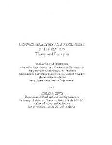
Convex Analysis and Non Linear Optimization Theory and Examples PDF
Preview Convex Analysis and Non Linear Optimization Theory and Examples
CONVEX ANALYSIS AND NONLINEAR OPTIMIZATION Theory and Examples JONATHAN M. BORWEIN Centre for Experimental and Constructive Mathematics Department of Mathematics and Statistics Simon Fraser University, Burnaby, B.C., Canada V5A 1S6 jborwein@cecm.sfu.ca http://www.cecm.sfu.ca/∼jborwein and ADRIAN S. LEWIS Department of Combinatorics and Optimization University of Waterloo, Waterloo, Ont., Canada N2L 3G1 aslewis@orion.uwaterloo.ca http://orion.uwaterloo.ca/∼aslewis To our families 2 Contents 0.1 Preface . . . . . . . . . . . . . . . . . . . . . . . . . . . . . . . 5 1 Background 7 1.1 Euclidean spaces . . . . . . . . . . . . . . . . . . . . . . . . . 7 1.2 Symmetric matrices . . . . . . . . . . . . . . . . . . . . . . . . 16 2 Inequality constraints 22 2.1 Optimality conditions . . . . . . . . . . . . . . . . . . . . . . . 22 2.2 Theorems of the alternative . . . . . . . . . . . . . . . . . . . 30 2.3 Max-functions and first order conditions . . . . . . . . . . . . 36 3 Fenchel duality 42 3.1 Subgradients and convex functions . . . . . . . . . . . . . . . 42 3.2 The value function . . . . . . . . . . . . . . . . . . . . . . . . 54 3.3 The Fenchel conjugate . . . . . . . . . . . . . . . . . . . . . . 61 4 Convex analysis 78 4.1 Continuity of convex functions . . . . . . . . . . . . . . . . . . 78 4.2 Fenchel biconjugation . . . . . . . . . . . . . . . . . . . . . . . 90 4.3 Lagrangian duality . . . . . . . . . . . . . . . . . . . . . . . . 103 5 Special cases 113 5.1 Polyhedral convex sets and functions . . . . . . . . . . . . . . 113 5.2 Functions of eigenvalues . . . . . . . . . . . . . . . . . . . . . 120 5.3 Duality for linear and semidefinite programming . . . . . . . . 126 5.4 Convex process duality . . . . . . . . . . . . . . . . . . . . . . 132 6 Nonsmooth optimization 143 6.1 Generalized derivatives . . . . . . . . . . . . . . . . . . . . . . 143 3 6.2 Nonsmooth regularity and strict differentiability . . . . . . . . 151 6.3 Tangent cones . . . . . . . . . . . . . . . . . . . . . . . . . . . 158 6.4 The limiting subdifferential . . . . . . . . . . . . . . . . . . . 167 7 The Karush-Kuhn-Tucker theorem 176 7.1 An introduction to metric regularity . . . . . . . . . . . . . . 176 7.2 The Karush-Kuhn-Tucker theorem . . . . . . . . . . . . . . . 184 7.3 Metric regularity and the limiting subdifferential . . . . . . . . 191 7.4 Second order conditions . . . . . . . . . . . . . . . . . . . . . 197 8 Fixed points 204 8.1 Brouwer’s fixed point theorem . . . . . . . . . . . . . . . . . . 204 8.2 Selection results and the Kakutani-Fan fixed point theorem . . 216 8.3 Variational inequalities . . . . . . . . . . . . . . . . . . . . . . 227 9 Postscript: infinite versus finite dimensions 238 9.1 Introduction . . . . . . . . . . . . . . . . . . . . . . . . . . . . 238 9.2 Finite dimensionality . . . . . . . . . . . . . . . . . . . . . . . 240 9.3 Counterexamples and exercises . . . . . . . . . . . . . . . . . . 243 9.4 Notes on previous chapters . . . . . . . . . . . . . . . . . . . . 249 9.4.1 Chapter 1: Background . . . . . . . . . . . . . . . . . . 249 9.4.2 Chapter 2: Inequality constraints . . . . . . . . . . . . 249 9.4.3 Chapter 3: Fenchel duality . . . . . . . . . . . . . . . . 249 9.4.4 Chapter 4: Convex analysis . . . . . . . . . . . . . . . 250 9.4.5 Chapter 5: Special cases . . . . . . . . . . . . . . . . . 250 9.4.6 Chapter 6: Nonsmooth optimization . . . . . . . . . . 250 9.4.7 Chapter 7: The Karush-Kuhn-Tucker theorem . . . . . 251 9.4.8 Chapter 8: Fixed points . . . . . . . . . . . . . . . . . 251 10 List of results and notation 252 10.1 Named results and exercises . . . . . . . . . . . . . . . . . . . 252 10.2 Notation . . . . . . . . . . . . . . . . . . . . . . . . . . . . . . 267 Bibliography 276 Index 290 4 0.1 Preface Optimization is a rich and thriving mathematical discipline. Properties of minimizers and maximizers of functions rely intimately on a wealth of tech- niques from mathematical analysis, including tools from calculus and its generalizations, topological notions, and more geometric ideas. The the- ory underlying current computational optimization techniques grows ever more sophisticated – duality-based algorithms, interior point methods, and control-theoreticapplicationsaretypicalexamples. Thepowerfulandelegant language of convex analysis unifies much of this theory. Hence our aim of writing a concise, accessible account of convex analysis and its applications and extensions, for a broad audience. For students of optimization and analysis, there is great benefit to blur- ring the distinction between the two disciplines. Many important analytic problems have illuminating optimization formulations and hence can be ap- proached through our main variational tools: subgradients and optimality conditions, the many guises of duality, metric regularity and so forth. More generally, the idea of convexity is central to the transition from classical analysis to various branches of modern analysis: from linear to nonlinear analysis, from smooth to nonsmooth, and from the study of functions to multifunctions. Thus although we use certain optimization models repeat- edly to illustrate the main results (models such as linear and semidefinite programming duality and cone polarity), we constantly emphasize the power of abstract models and notation. Good reference works on finite-dimensional convex analysis already exist. Rockafellar’s classic Convex Analysis [149] has been indispensable and ubiq- uitous since the 1970’s, and a more general sequel with Wets, Variational Analysis [150], appeared recently. Hiriart-Urruty and Lemar´echal’s Convex Analysis and Minimization Algorithms [86] is a comprehensive but gentler introduction. Our goal is not to supplant these works, but on the contrary to promote them, and thereby to motivate future researchers. This book aims to make converts. We try to be succinct rather than systematic, avoiding becoming bogged down in technical details. Our style is relatively informal: for example, the text of each section sets the context for many of the result statements. We value the variety of independent, self-contained approaches over a single, unified, sequential development. We hope to showcase a few memorable principles rather than to develop the theory to its limits. We discuss no 5 algorithms. We point out a few important references as we go, but we make no attempt at comprehensive historical surveys. Infinite-dimensional optimization lies beyond our immediate scope. This is for reasons of space and accessibility rather than history or application: convex analysis developed historically from the calculus of variations, and has important applications in optimal control, mathematical economics, and other areas of infinite-dimensional optimization. However, rather like Hal- mos’s Finite Dimensional Vector Spaces [81], ease of extension beyond fi- nite dimensions substantially motivates our choice of results and techniques. Wherever possible, wehavechosen aprooftechnique thatpermitsthoseread- ers familiar with functional analysis to discover for themselves how a result extends. We would, in part, like this book to be an entr´ee for mathemati- cians to a valuable and intrinsic part of modern analysis. The final chapter illustrates some of the challenges arising in infinite dimensions. This book can (and does) serve as a teaching text, at roughly the level of first year graduate students. In principle we assume no knowledge of real analysis, although in practice we expect a certain mathematical maturity. Whilethemainbodyofthetext isself-contained, eachsectionconcludes with anoftenextensive set ofoptionalexercises. Theseexercises fallintothreecat- egories, marked with zero, one or two asterisks respectively: examples which illustrate the ideas in the text or easy expansions of sketched proofs; im- portant pieces of additional theory or more testing examples; longer, harder examples or peripheral theory. WearegratefultotheNaturalSciences andEngineeringResearchCouncil of Canada for their support during this project. Many people have helped improve the presentation of this material. We would like to thank all of them, but in particular Guillaume Haberer, Claude Lemar´echal, Olivier Ley, Yves Lucet, Hristo Sendov, Mike Todd, Xianfu Wang, and especially Heinz Bauschke. Jonathan M. Borwein Adrian S. Lewis Gargnano, Italy September, 1999 6 Chapter 1 Background 1.1 Euclidean spaces We begin by reviewing some of the fundamental algebraic, geometric and analytic ideas we use throughout the book. Our setting, for most of the book, is an arbitrary Euclidean space E, by which we mean a finite- dimensional vector space over the reals R, equipped with an inner product (cid:2)·,·(cid:3). We would lose no generality if we considered only the space Rn of real (column) n-vectors (with its standard inner product), but a more abstract, coordinate-free notation is often more flexible and elegant. (cid:1) We define the norm of any point x in E by (cid:4)x(cid:4) = (cid:2)x,x(cid:3), and the unit ball is the set B = {x ∈ E|(cid:4)x(cid:4) ≤ 1}. Any two points x and y in E satisfy the Cauchy-Schwarz inequality |(cid:2)x,y(cid:3)| ≤ (cid:4)x(cid:4)(cid:4)y(cid:4). We define the sum of two sets C and D in E by C +D = {x+y |x ∈ C, y ∈ D}. The definition of C −D is analogous, and for a subset Λ of R we define ΛC = {λx|λ ∈ Λ, x ∈ C}. Given another Euclidean space Y, we can consider the Cartesian product EuclideanspaceE×Y,withinnerproductdefinedby(cid:2)(e,x),(f,y)(cid:3) = (cid:2)e,f(cid:3)+ (cid:2)x,y(cid:3). 7 8 Background We denote the nonnegative reals by R . If C is nonempty and satisfies + R C = C we call it a cone. (Notice we require that cones contain 0.) + Examples are the positive orthant Rn = {x ∈ Rn |each x ≥ 0}, + i and the cone of vectors with nonincreasing components Rn = {x ∈ Rn |x ≥ x ≥ ... ≥ x }. ≥ 1 2 n The smallest cone containing a given set D ⊂ E is clearly R D. + The fundamental geometric idea of this book is convexity. A set C in E is convex if the line segment joining any two points x and y in C is contained in C: algebraically, λx+(1−λ)y ∈ C whenever 0 ≤ λ ≤ 1. An easy exercise shows that intersections of convex sets are convex. Given any set D ⊂ E, the linear span of D, denoted span(D), is the smallest linear subspace containing D. It consists exactly of all linear com- binations of elements of D. Analogously, the convex hull of D, denoted conv(D), is the smallest convex set containing D. It consists exactly of all convex combinations of elements of D, that is to say points of the form (cid:2) (cid:2) m λ xi, where λ ∈ R and xi ∈ D for each i, and λ = 1 (see Exercise i=1 i i + i 2). The language of elementary point-set topology is fundamental in opti- mization. A point x lies in the interior of the set D ⊂ E (denoted intD) if there is a real δ > 0 satisfying x + δB ⊂ D. In this case we say D is a neighbourhood of x. For example, the interior of Rn is + Rn = {x ∈ Rn |each x > 0}. ++ i We say the point x in E is the limit of the sequence of points x1,x2,... in E, written xi → x as i → ∞ (or lim xi = x), if (cid:4)xi −x(cid:4) → 0. The closure i→∞ of D is the set of limits of sequences of points in D, written clD, and the boundary of D is clD\intD, written bdD. The set D is open if D = intD, and is closed if D = clD. Linear subspaces of E are important examples of closed sets. Easy exercises show that D is open exactly when its complement Dc is closed, and that arbitrary unions and finite intersections of open sets are open. The interior of D is just the largest open set contained in D, while clD is the smallest closed set containing D. Finally, a subset G of D is open in D if there is an open set U ⊂ E with G = D ∩U. §1.1 Euclidean spaces 9 Much of the beauty of convexity comes from duality ideas, interweaving geometry and topology. The following result, which we prove a little later, is both typical and fundamental. Theorem 1.1.1 (Basic separation) Suppose that the set C ⊂ E is closed and convex, and that the point y does not lie in C. Then there exist real b and a nonzero element a of E satisfying (cid:2)a,y(cid:3) > b ≥ (cid:2)a,x(cid:3) for all points x in C. Sets in E of the form {x|(cid:2)a,x(cid:3) = b} and {x|(cid:2)a,x(cid:3) ≤ b} (for a nonzero element a of Eand realb) arecalled hyperplanes andclosed halfspacesrespec- tively. In this language the above result states that the point y is separated from the set C by a hyperplane: in other words, C is contained in a certain closed halfspace whereas y is not. Thus there is a ‘dual’ representation of C as the intersection of all closed halfspaces containing it. The set D is bounded if there is a real k satisfying kB ⊃ D, and is compact if it is closed and bounded. The following result is a central tool in real analysis. Theorem 1.1.2 (Bolzano-Weierstrass) Any bounded sequence in E has a convergent subsequence. Just as for sets, geometric and topological ideas also intermingle for the functions we study. Given a set D in E, we call a function f : D → R continuous (on D) if f(xi) → f(x) for any sequence xi → x in D. In this case it easy to check, for example, that for any real α the level set {x ∈ D |f(x) ≤ α} is closed providing D is closed. Given another Euclidean space Y, we call a map A : E → Y linear if any points x and z in E and any reals λ and µ satisfy A(λx + µz) = λAx + µAz. In fact any linear function from E to R has the form (cid:2)a,·(cid:3) for some element a of E. Linear maps and affine functions (linear functions plus constants) are continuous. Thus, for example, closed halfspaces are indeed closed. A polyhedron is a finite intersection of closed halfspaces, and is therefore both closed and convex. The adjoint of the map A above is the linear map A∗ : Y → E defined by the property (cid:2)A∗y,x(cid:3) = (cid:2)y,Ax(cid:3), for all points x in E and y in Y (whence A∗∗ = A). The null space of A is N(A) = {x ∈ E|Ax = 0}. The inverse image of a set H ⊂ Y is the set A−1H = {x ∈ E | Ax ∈ H} (so 10 Background for example N(A) = A−1{0}). Given a subspace G of E, the orthogonal complement of G is the subspace G⊥ = {y ∈ E|(cid:2)x,y(cid:3) = 0 for all x ∈ G}, so called because we can write E as a direct sum G⊕G⊥. (In other words, any element of E can be written uniquely as the sum of an element of G and an element of G⊥.) Any subspace satisfies G⊥⊥ = G. The range of any linear map A coincides with N(A∗)⊥. Optimization studies properties of minimizers and maximizers of func- tions. Given a set Λ ⊂ R, the infimum of Λ (written infΛ) is the greatest lower bound on Λ, and the supremum (written supΛ) is the least upper bound. To ensure these are always defined, it is natural to append −∞ and +∞ to the real numbers, and allow their use in the usual notation for open and closed intervals. Hence inf∅ = +∞ and sup∅ = −∞, and for example (−∞,+∞] denotes the interval R∪{+∞}. We try to avoid the appearance of +∞−∞, but when necessary we use the convention +∞−∞ = +∞, so that any two sets C and D in R satisfy infC +infD = inf(C+D). We also adopt the conventions 0·(±∞) = (±∞)·0 = 0. A (global) minimizer of a function f : D → R is a point x¯ in D at which f attains its infimum inff = inff(D) = inf{f(x)|x ∈ D}. D In this case we refer to x¯ as an optimal solution of the optimization problem inf f. D For a positive real δ and a function g : (0,δ) → R, we define liminfg(t) = lim inf g, and t↓0 t↓0 (0,t) limsupg(t) = limsupg. t↓0 t↓0 (0,t) The limit lim g(t) exists if and only if the above expressions are equal. t↓0 The question of the existence of an optimal solution for an optimization problem is typically topological. The following result is a prototype. The proof is a standard application of the Bolzano-Weierstrass theorem above. Proposition 1.1.3 (Weierstrass) Suppose that the set D ⊂ E is nonempty and closed, and that all the level sets of the continuous function f : D → R are bounded. Then f has a global minimizer.
The list of books you might like

The 48 Laws of Power

The Mountain Is You

The 48 Laws of Power

A Thousand Boy Kisses

Satellite technology: principles and applications

Bureau for International Narcotics and Law Enforcement Affairs

The Fighting Tomahawk An Illustrated Guide to Using the Tomahawk and Long Knife as Weapons

COMESA 273: Textile fibres - Determination of breaking force and elongation at break of individual fibres

COMESA 265-1: Textiles — Burning behaviour of bedding items —Part 1:General test methods for the ignitability by a smouldering cigarette
Your Turn Answer Key - Houghton Mifflin Harcourt
Modern Asian Studies 2006: Vol 40 Index

Svoboda-2006-33
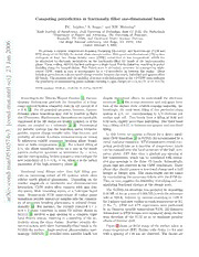
Competing periodicities in fractionally filled one-dimensional bands
C. Indice de autores

Opportunities in fashion careers

My Sister, My Love

BVCM002573 M-30
The Jade God by Alan Sullivan
California Accidental Release Prevention (CalARP) Program

Antibiotic Review Kit - Hospital (ARK-hospital)
California adrift internationally: resetting course for the - Aabri.com
