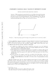
Comparing maximal mean values on different scales

0.4 MB·English

by  Thomas Havenith

COMPARING MAXIMAL MEAN VALUES ON DIFFERENT SCALES
THOMAS HAVENITH AND SEBASTIAN SCHOLTES
Abstract. When computing the average speed of a car over different time periods from given
GPS data, it is conventional wisdom that the maximal average speed over all time intervals of
fixed length decreases if the interval length increases. However, this intuition is wrong. This can
be easily seen by the example in Figure 1 for the two time periods T <S. We investigate this
phenomenon and make rigorous in which sense this intuition is still true.
5
1
0
2

n
a
J

0
2

]
M
G
.
h
t
a Figure 1. Maximal average speeds for larger time periods are not necessarily smaller.
m
[

1 In many applications, rates are measured as average velocities; for instance the speed monitored
v
by Speed Check Services SPECS in the UK, capacities of rides in amusement parks and the drift
1
9 velocity of electrons are obtained in this way [Smi12, Ahm97, Gri99]. In other fields mean values
3 over different time intervals and their relation are important:
6
0 • An athlete has a high heart rate during a competition and maybe even a very high heart
.
1 rate for a small time during this contest, but having a similar heart rate for a whole
0 week would result in serious health problems.
5
• While approximately 10 percent of people that are exposed to a radiation dose of 1 Sv
1
: over a short time period die from light radiation poisoning in the first 30 days [Har11,
v
p.400], this is also the maximal dose allowed for NASA astronauts over their career,
i
X [NAS08, p.7].
r • Certain materials, for example a power line, can endure fairly high stresses, currents etc.
a
for a small time interval, but the average load on a larger time scale has to be much
smaller. Another illustration for the effect of the time scale is the phenomenon of creep
[MC99].
All these examples show that one expects maximal mean values to become smaller as the
interval size decreases. We study mean values (in the discrete as well as in the continuous setting)
with regard to this property and find that it is not true in general (Lemmata 3 and 8), but that
it is true if one compares the maximal mean value over all regions of size T with those taken on
regions of size d·T for d ∈ N (Lemmata 3 and 7).
Date: January 27, 2015.
2010 Mathematics Subject Classification. 46B25; 62P30, 46A45, 47A30.
Key words and phrases. mean value, arithmetic mean, norm, Lp norm.
1
2 THOMASHAVENITHANDSEBASTIANSCHOLTES
1. Discrete setting
Let (cid:96)∞ be the space of bounded real sequences. For x ∈ (cid:96)∞, p ∈ (0,∞) and n ∈ N we define
j+(n−1)
(cid:16)1 (cid:88) (cid:17)1
(cid:107)x(cid:107) := sup |x |p p.
∞,p,n j∈N n i
i=j
Lemma 1 (For p ∈ [1,∞) the mapping (cid:107)·(cid:107) is an equivalent norm to (cid:107)·(cid:107) ).
∞,p,n ∞
Let p ∈ [1,∞), n ∈ N. Then (cid:107)·(cid:107) is a norm on (cid:96)∞ with
∞,p,n
−1
n p(cid:107)x(cid:107) ≤ (cid:107)x(cid:107) ≤ (cid:107)x(cid:107) .
∞ ∞,p,n ∞
Proof. Clearly (cid:107)·(cid:107) is positively homogenous of degree one and (cid:107)x(cid:107) ≥ 0 with equality if
∞,p,n ∞,p,n
and only if x = 0. From the triangle inequality of the p-norm in Euclidean n-space we obtain the
triangle inequality for (cid:107)·(cid:107) . Additionally, we obtain
∞,p,n
j+(n−1)
n−p1(cid:107)x(cid:107)∞ = (cid:16)n1(cid:107)x(cid:107)p∞(cid:17)p1 ≤ (cid:107)x(cid:107)∞,p,n = sju∈Np(cid:16)n1 (cid:88) |xi|p(cid:17)p1 ≤ (cid:16)n1n(cid:107)x(cid:107)p∞(cid:17)p1 = (cid:107)x(cid:107)∞.
i=j
(cid:3)
This means that the spaces ((cid:96)∞,(cid:107)·(cid:107) ) are non-reflexive Banach spaces with the same
∞,p,n
topology as the standard (cid:96)∞.
Lemma 2 (Inequality for norms).
Let α ∈ N with n = (cid:80)d α . Then for all p ∈ [1,∞) and x ∈ (cid:96)∞ we have that
i l=1 l
d
(cid:107)x(cid:107)p ≤ (cid:88) αl(cid:107)x(cid:107)p .
∞,p,n n ∞,p,αl
l=1
Proof. Let j ∈ N, ε > 0 such that (cid:107)x(cid:107)p −ε ≤ 1 (cid:80)j+(n−1)xp. Then
∞,p,n n i=j i
(cid:107)x(cid:107)p −ε ≤ 1 j+(cid:88)(n−1)xp = 1 (cid:88)d j+(cid:80)lk−=11(cid:88)αk+(αl−1)xp ≤ 1 (cid:88)d α (cid:107)x(cid:107)p .
∞,p,n n i n i n l ∞,p,αl
i=j l=1 i=j+(cid:80)l−1 α l=1
k=1 k
(cid:3)
Lemma 3 (Norms (cid:107)·(cid:107) of multiples of n are ordered).
∞,p,dn
Let m,n ∈ N and n ≤ m.
• If n is a factor of m, i.e. m = dn for d ∈ N then
(cid:107)x(cid:107) = (cid:107)x(cid:107) ≤ (cid:107)x(cid:107) for all x ∈ (cid:96)∞.
∞,p,dn ∞,p,m ∞,p,n
• If n is no factor of m then there are x,y ∈ (cid:96)∞ such that
(cid:107)x(cid:107) < (cid:107)x(cid:107) and (cid:107)y(cid:107) < (cid:107)y(cid:107) .
∞,p,n ∞,p,m ∞,p,m ∞,p,n
Proof. If we choose all α = n in Lemma 2 we immediately obtain the first item. For the second
l
item define x(n) ∈ (cid:96)∞ by x(n) = 1 if i ∈ {(d−1)n+1 | d ∈ N} and x(n) = 0 otherwise. Then
i i
1 d d
(cid:107)x(n)(cid:107)p = < ≤ = (cid:107)x(n)(cid:107)p
∞,p,n n dn−1 (d−1)n+j ∞,p,(d−1)n+j
for j = 1,...,n−1 and d ∈ N. Note that the natural numbers of the form m = (d−1)n+j for
j = 1,...,n−1, d ∈ N are exactly those which are either smaller than n or such that n is no
factor of m. This proves the proposition as we obtain the opposite inequality by interchanging
the roles of m and n. (cid:3)
In the following Lemma we show that counterexamples, however, cannot be too bad.
COMPARING MAXIMAL MEAN VALUES ON DIFFERENT SCALES 3
Lemma 4 (Counterexamples cannot be too bad).
Let p ∈ [1,∞), n < m. Then for all x ∈ (cid:96)∞ we have that
((cid:98)m(cid:99)+1)n
(cid:107)x(cid:107)p ≤ n (cid:107)x(cid:107)p ≤ 2(cid:107)x(cid:107)p .
∞,p,m m ∞,p,n ∞,p,n
Proof. Choose d := (cid:98)m(cid:99) and ε > 0. Then there is j ∈ N such that
n
j+(m−1) j+((d+1)n−1)
1 (cid:88) 1 (cid:88)
(cid:107)x(cid:107)p −ε ≤ |x |p ≤ |x |p
∞,p,m m i m i
i=j i=j
(d+1)n (d+1)n
≤ (cid:107)x(cid:107)p ≤ (cid:107)x(cid:107)p
m ∞,p,(d+1)n m ∞,p,n
according to Lemma 3. (cid:3)
2. Continuous setting
Let f : RN → R be a function. For V > 0, p ∈ (0,∞) we define
(cid:16) 1 (cid:90) (cid:17)1
(cid:107)f(cid:107) := sup |f(x)|pdx p.
p,V |Ω|
Ω⊂RN open Ω
Ωconvex
|Ω|=V
NotethatthisnormbearsaresemblancetotheHardy-Littlewoodmaximalfunctionfromharmonic
analysis. If we denote the space of all functions f : RN → R with f = 0 a.e. by N we can define
Lp := {f : RN → R | (cid:107)f(cid:107) < ∞}/N.
V p,V
By a slight abuse of notation we also want to consider (cid:107)·(cid:107) as a mapping from Lp to R in the
p,V V
obvious manner.
Lemma 5 (For p ∈ [1,∞) the mapping (cid:107)·(cid:107) is a norm on Lp ).
p,V V
Let p ∈ [1,∞), V > 0. Then (cid:107)·(cid:107) is a norm on Lp .
p,V V
Proof. Clearly (cid:107)·(cid:107) is positively homogenous of degree one and (cid:107)f(cid:107) ≥ 0 with equality if and
p,V p,V
only if f = 0 a.e.. Now, the triangle inequality for Lp proves the triangle inequality for (cid:107)·(cid:107) . (cid:3)
p,V
Lemma 6 (Inequality for norms).
Let α > 0 with V = (cid:80)d α . Then for all p ∈ [1,∞), V > 0 and f ∈ Lp holds
i l=1 l V
d
(cid:107)f(cid:107)p ≤ (cid:88) αl(cid:107)f(cid:107)p .
p,V V p,αl
l=1
Proof. Step 1 Let ε > 0 and Ω ⊂ RN be open and connected such that (cid:107)f(cid:107)p − ε ≤
p,V
1 (cid:82) |f(x)|pdx. According to Step 2 there is a hyperplane that cuts Ω into two convex sets Ω
|Ω| Ω 1
and Ω˜ with |Ω | = α and |Ω˜ | = (cid:80)d α . Now iterating this procedure with Ω˜ we finally
1 1 1 1 l=2 l 1
obtain d open convex sets Ω with |Ω | = α and Ω = (cid:83)d Ω ∪A, where HN(A) = 0, as A is
i i i l=1 i
contained in a finite union of hyperplanes. Therefore
(cid:90) d (cid:90) d
(cid:107)f(cid:107)p −ε ≤ 1 |f(x)|pdx = 1 (cid:88) |f(x)|pdx ≤ 1 (cid:88)α (cid:107)f(cid:107)p .
p,V |Ω| |Ω| |Ω| l p,αl
Ω l=1 Ωi l=1
Step 2 Let Ω be an open convex set and α+β = |Ω| for α,β > 0. If we define
Ω := {x ∈ Ω | x = s}
s 1
we know by Cavalieri’s Principle (a special case of Fubini’s Theorem) that the function ϕ(t) :=
(cid:82)t
|Ω |ds measures the volume of the set Ω intersected with the open half-space below (in e
−∞ s 1
direction) the hyperplane {x ∈ RN | x = t}. Additionally lim ϕ(t) = 0, lim ϕ(t) = |Ω|
1 t→−∞ t→∞
and ϕ is continuous. Therefore the intermediate value theorem yields the existence of a t such
0
that Ω = (cid:83) Ω and Ω˜ = (cid:83) Ω are open convex sets (as intersection of two such
1 t∈(−∞,t0) t 1 t∈(t0,∞) t
sets) and |Ω | = α and |Ω˜ | = |Ω|−α = β. (cid:3)
1 1
4 THOMASHAVENITHANDSEBASTIANSCHOLTES
Lemma 7 (Norms (cid:107)·(cid:107) of multiples of V are ordered).
p,d·V
Let p ∈ [1,∞), V > 0 and d ∈ N. Then
(cid:107)f(cid:107) ≤ (cid:107)f(cid:107) for all f ∈ Lp .
p,d·V p,V V
Proof. If we chose all α = V in Lemma 6 we directly obtain the result. (cid:3)
l
Lemma 8 (For N = 1, T < S and T no factor of S the norms are not ordered).
Let N = 1, p ∈ [1,∞) and T,S > 0, T < S such that T is no factor of S. Then there are
f,g ∈ Lp such that
T
(cid:107)f(cid:107) < (cid:107)f(cid:107) and (cid:107)g(cid:107) < (cid:107)g(cid:107) .
p,T p,S p,S p,T
Proof. Let T < S such that T is not a factor of S, i.e. S (cid:54)∈ N. Write d := (cid:98)S(cid:99). Then it is possible
T T
to choose ε > 0 such that (d+1)ε < S −dT. Let ψ (x) be a bump function of Lp mass 1 with
ε
support in (0,ε). Then f(x) = (cid:80)d ψ (x−i(T +ε)) is an Lp function and
i=0 ε T
1 d+1
(cid:107)f(cid:107)p = < = (cid:107)f(cid:107)p ,
p,T T S p,S
because S < (cid:98)S(cid:99)+1. On the other hand, g = ψ ∈ Lp yields
T T ε T
1 1
(cid:107)g(cid:107)p = < = (cid:107)g(cid:107)p .
p,S S T p,T
(cid:3)
Corollary 9 (Counterexamples cannot be too bad).
Let p ∈ [1,∞), T < S. Then for all f ∈ Lp holds
S
((cid:98)S(cid:99)+1)T
(cid:107)f(cid:107)p ≤ T (cid:107)f(cid:107)p ≤ 2(cid:107)f(cid:107)p.
p,S S T T
Proof. Choose d := (cid:98)S(cid:99) and ε > 0 such that (cid:107)f(cid:107)p −ε ≤ 1 (cid:82) |f(t)|pdt. Then we can extend Ω
T p,S S Ω
convexly to an open Ω˜ with Ω ⊂ Ω˜ and |Ω˜| = (d+1)T. This can for example be done by taking
the convex hull Ω˜ of Ω and a point y moving along a normal at a fixed point y ∈ ∂Ω. By an
y
argument similar to that in the proof of Lemma 6 Step 2, we see that x can be chosen in such a
way that |Ω˜ | = (d+1)T. Now
y
(cid:90) (cid:90)
1 1 (d+1)T (d+1)T
(cid:107)f(cid:107)p −ε ≤ |f(t)|pdt ≤ |f(t)|pdt ≤ (cid:107)f(cid:107)p ≤ (cid:107)f(cid:107)p
p,S S Ω S Ω˜ S (d+1)T S T
by Lemma 7. (cid:3)
References
[Ahm97] Reza H. Ahmadi, Opportunities for simulation in amusement parks, Oper. Res. 45 (1997), no. 1, 1–13.
[Gri99] David Griffiths, Introduction to electrodynamics, Prentice-Hall, 1999.
[Har11] Gavin D. J. Harper, Green Health: An A-to-Z Guide, ch. Radiation Sources, pp. 374–401, SAGE, 2011.
[MC99] M. A. Meyers and K. K. Chawla, Mechanical Behavior of Materials, Cambridge University Press, 1999.
[NAS08] NASA, Space Faring: The Radiation Challenge Introduction and Module 1: Radiation, Educator Guide
EP-2008-08-116-MSFC, NASA, 2008.
[Smi12] B.D.V. Smith, Vehicle speed monitoring system, US Patent 8,189,048, 2012.
Thomas Havenith, Infrastrukturplanung (I.ETZ 1), DB Energie GmbH, Pfarrer-Perabo-Platz 2,
60326 Frankfurt am Main, Germany
E-mail address: [email protected]
URL: http://www.dbenergie.de/
Sebastian Scholtes, Institut für Mathematik, RWTH Aachen University, Templergraben 55, 52062
Aachen, Germany
E-mail address: [email protected]
URL: http://www.instmath.rwth-aachen.de/~scholtes/home/