PDF Vs CDF 2022: Most The Difference For Your Choice

PDF Vs CDF is both types of files that store data. PDFs are usually used to store documents, while CDFs are used to store data sets.

There are two main types in the world of data: continuous and discrete. Continuous data can be measured in any unit, while discrete data can only be measured in specific units. One type of continuous data is probability density function (PDF), while the other is cumulative distribution function (CDF).

Contents

1 The Cumulative Distribution Function (CDF)
2 Probability Density Function (PDF)
3 CDF vs. PDF: What’s the Difference?
4 The Relationship Between a CDF and a PDF
5 FAQ
6 Conclusion

The Cumulative Distribution Function (CDF)

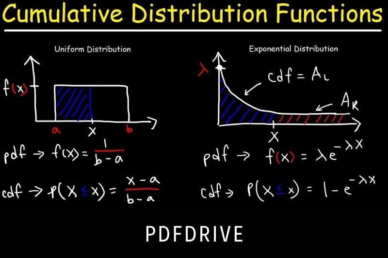
Cumulative distribution function (CDF) is the probability that random variables, such as X will have a value lower than or equal to x.

If you roll a die, your chances of getting 1, 2, 3, 4, 5, 5, or 6 are 16.667% (=1/6). Cumulative distribution function (CDF of 1) is the probability that your next roll will have a value lower than or equal to 1 and equals 16.667%. There is only one way to get 1.

Cumulative distribution function (CDF2) of 2 indicates the likelihood that the next roll will have a value lower than or equal to 2 and equals 33.33%. There are two ways to get a two or lower. The cumulative distribution function (CDF6) of 6 is 100%.

Cumulative distribution function (CDF6) of 6 indicates the likelihood that the next roll will have a value lower than or equal to 6 and equals 100% for all possible results.

Probability Density Function (PDF)

The probability density function (PDF) is the probability that an unknown random variable, such as X will have a value exactly equivalent to x. The difference between the cumulative distribution (CDF) and the probability density (PDF) is obvious. Here, the focus is on one value.

However, for the cumulative distribution function, we are only interested in the probability that the value is equal to or lower than the given value. Also known as the probability density function, it is also called the probability mass function. Do not be alarmed if you come across the probability mass function.

If you roll a die, for example, the probability that you will get 1, 2, 3, 4, 5, 5, or 6 is 16.667% (=1/6). 16.667% is the probability density function (PDF), or the probability of getting exactly 2.

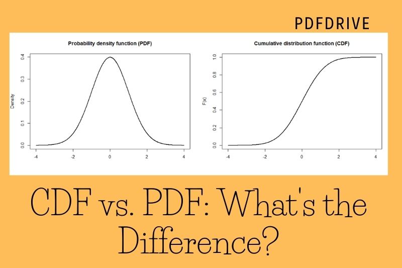
CDF vs. PDF: What’s the Difference?

Random Variables

Before creating a PDF or a CDF, we must first understand random variables.

A random variable (usually denoted as “X”) is a variable whose numbers result from some random process. There are two types: continuous and discrete random variables.

Discrete Random Variables

A discrete random variable can only take on a limited number of distinct values, such as 0, 1, 2, 3, 4, 5, 5…100, 1,000,000, etc. Examples of discrete random variables are:

After being flipped 20 times, the number of coins that land on tails.

After being rolled 100 times, the number of times a dice hits the number 4 is its number.

Continuous Random Variables

Continuous random variables can have infinite numbers of possible values. Examples of continuous random variables are:

The height of a person
Animal weight
To run a mile takes time.

A person’s height could range from 60.2 inches to 65.2344 inches to 70.431222 inches and so on. There are many possible height values.

Rule of thumb: If you can count the outcomes, you have a discrete random variable. (e.g., The number of coins that land on heads. If you can measure the outcome of the coin landing on heads, then you’re working with a continuous random variable. measuring, height, weight, time, etc.)

Probability Density Functions

A probability density function (pdf) tells us how likely a random variable will take on a particular value.

Let’s say we roll a single dice. Let x be the number of dice that land on the table. The probability density function for the outcome is described as follows:

P(x < 1) : 0

P(x = 1) : 1/6

P(x = 2) : 1/6

P(x = 3) : 1/6

P(x = 4) : 1/6

P(x = 5) : 1/6

P(x = 6) : 1/6

P(x > 6) : 0

This is an example of a discrete random variable since x cannot take integer values.

We cannot use a PDF to represent a continuous random variable. The probability that x will take on any specific value is zero.

Let’s say, for example, we want to find out the likelihood that a burger at a restaurant will weigh a quarter-pound (0.25 pounds). Weight is a continuous variable that can take on infinite values.

A given burger could weigh 0.250001 pounds or 0.24 pounds or 0.2488 pounds. It is unlikely that a given hamburger will weigh exactly 0.25 pounds.

Cumulative Distribution Functions

The cumulative distribution function (CDF), which tells us how likely a random variable will take on a value of less than or equaling x, is called a cumulative distribution function.

Let’s say we roll a single dice. Let x be the number of dice that land on the table. The cumulative distribution function for the outcome can then be described as:

P(x <= 0) : 0

P(x <= 1) : 1/6

P(x <= 2) : 2/6

P(x <= 3) : 3/6

P(x <= 4) : 4/6

P(x <= 5) : 5/6

P(x <= 6) : 6/6

P(x > 6) : 0

You will notice that the probability of x being less than or equal to 6 is 6/6. This is equal to 1. This is because the dice can land on 1, 2, 3, 4, 5, 6, or 6 with 100% probability.

Although this example is based on a discrete random variable (or a continuous density function), it can generate a continuous random variable.

These properties are found in cumulative distribution functions:

Zero probability that a random variable will take on a smaller value than its smallest value. Zero is the probability that a die will land on a number less than 1.

One is the probability that a random variable will take on a smaller or greater value than its maximum value. One is the probability that a die lands on one of these numbers. It must land on one or more of these numbers.

The CDF is never decreasing. The probability of a dice landing on a number lower than or equal to 1 is 1/6. 2/6 is the probability it will land on a number lower than or equal to 2, and 3/6 is the probability of land on numbers less or equal to 3.

The cumulative probability of a dice landing on a number less than or equal to 1 is 1/6, the probability that it lands on a number less than or equal to 2 is 2/6, and so forth.

Similar: An ogive graph can visualize a cumulative distribution function.

The Relationship Between a CDF and a PDF

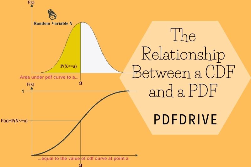
A probability density function (pdf), in technical terms, is the derivative of a cumulative function (CDF).

The area under the curve for a pdf between negative infinite and x is equal to the CDF.

A statistical textbook provides a detailed explanation of the relationship between pdf and CDF.

Some relevant articles:

FAQ

Is PDF the derivative of CDF?

If it exists, the probability density function F(x), abbreviated PDF, is the derivative from the CDF. A distribution function, FX(x), describes every random variable X.

What is the derivative of a PDF?

The probability density function (pdf), f(x), of a continuous random variable is defined as the derivative F(x)=ddxF[x]. Two important properties of the pdf f (x) are: f(x),>=0 for all x.

Is a PDF continuous?

Probability density function (PDF), a statistical expression, is used to define a probability distribution (the likelihood that an outcome will occur) for discrete random variables (e.g., stock or ETF) rather than a continuous random variable.

What is CDF in probability?

Probability theory and statistics use the cumulative distribution function (CDF), or just distribution function, to describe the probability that a real-valued random variable will have less or equal value.

Conclusion

There are many benefits to using PDFs over CDs, and the most important is that PDFs are searchable, while CDs are not. For this reason, it is generally recommended that you use PDFs whenever possible. Thanks for reading!