Measurement of inclusive two-particle angular correlations in pp collisions with the ATLAS detector PDF
Preview Measurement of inclusive two-particle angular correlations in pp collisions with the ATLAS detector
Published for SISSA by Springer Received: March 15, 2012 Accepted: May 10, 2012 Published: May 31, 2012 J Measurement of inclusive two-particle angular H correlations in pp collisions with the ATLAS detector E at the LHC P 0 5 ( 2 The ATLAS collaboration 0 E-mail: atlas.publications@cern.ch 1 2 Abstract: We present a measurement of two-particle angular correlations in proton- √ ) proton collisions at s = 900GeV and 7TeV. The collision events were collected during 2009 and 2010 with the ATLAS detector at the Large Hadron Collider using a single-arm 1 minimum bias trigger. Correlations are measured for charged particles produced in the 5 kinematic range of transverse momentum p > 100MeV and pseudorapidity |η| < 2.5. T 7 A complex structure in pseudorapidity and azimuth is observed at both collision ener- gies. Results are compared to pythia 8 and herwig++ as well as to the AMBT2B, DW and Perugia 2011 tunes of pythia 6. The data are not satisfactorily described by any of these models. Keywords: Hadron-Hadron Scattering Open Access, Copyright CERN, doi:10.1007/JHEP05(2012)157 for the benefit of the ATLAS collaboration Contents 1 Introduction 1 2 Definition of the two-particle correlation 2 3 The ATLAS detector 4 4 Monte Carlo models 5 J 5 Data samples and event selection 7 H E 6 Correction procedure 8 P 7 Statistical and systematic uncertainties 11 0 7.1 Statistical uncertainty 11 5 7.2 Uncertainties on the efficiencies 11 ( 7.3 Uncertainty due to lack of closure using Monte Carlo samples 11 2 8 Results and discussion 13 0 8.1 Projections in ∆η and ∆φ 14 1 9 Summary and conclusions 20 2 ) The ATLAS collaboration 24 1 5 7 1 Introduction Several phenomenological models have been formulated in order to describe the dynam- ics of multi-particle production in high-energy hadron collisions. Examples include the string [1] and cluster [2] models, but all have proven to be incomplete since they provide only limited explanations for the observed production of soft particles. The study of corre- lations between final-state particles is a powerful method for investigating the underlying mechanisms of particle production, as demonstrated by previous experiments [3–5]. Phe- nomenological models of soft particle production are encapsulated in a variety of different Monte Carlo (MC) generators. Particle correlation measurements provide useful input for discriminating between such models and for tuning their parameters in order to better describe non-perturbative physics. Model features that are sensitive to measurements of correlations include fragmentation, resonance decays, multi-parton interactions, and the emergence of jets. The measurement of correlated particle production in proton-proton collisions is also very useful for studies of heavy ion collisions; any deviation in the latter fromthebehaviourseenintheformercanbeattributedtothefactthatpartonsexperience – 1 – additional interactions, and other collective effects, in the hot and dense medium present in heavy ion collisions. This study focuses on the two-particle angular correlations in pseudorapidity, η, and azimuthalangle,φ,usingproton-protoncollisiondatacollectedbytheATLASexperiment1 at the Large Hadron Collider (LHC). A measurement of the inclusive two-particle angular correlation function is performed for charged particles produced in the kinematic region defined by p > 100 MeV2 and |η| < 2.5 in proton-proton collisions at centre-of-mass T √ collision energies of s = 900GeV and 7TeV. For the 7TeV centre-of-mass energy, an additional region of phase space is considered for which the charged-particle multiplicity per event is at least twenty. J The paper is organised as follows: the two-particle correlation definition used here is H described in section 2, while a brief description of the ATLAS detector is presented in E section 3. Section 4 summarises the different Monte Carlo models used in this study and P thedatasamplesandeventselectionaredescribedinsection5. Insection6thedata-driven procedure for unfolding the effect of the detection apparatus from the physics is presented. 0 The sources of systematic uncertainty affecting the analysis are discussed in section 7. 5 Finally, the corrected two-particle angular correlation functions and a comparison to a ( variety of different Monte Carlo predictions are shown in section 8. 2 0 2 Definition of the two-particle correlation 1 The correlation function is defined using two different distributions that are dependent on 2 η and φ. The foreground distribution, F(n ,∆η,∆φ), describes the angular separation in ch ) azimuth(∆φ)andpseudorapidity(∆η)betweenpairsofparticlesemittedinthesameevent 1 of charged multiplicity n . F(n ,∆η,∆φ) is defined for all events with n greater than ch ch ch 5 one and contains correlations due to both the underlying physics processes and detector effects such as geometrical acceptance. The expression for F(n ,∆η,∆φ) is given by 7 ch (cid:42) (cid:43) 2 (cid:88)(cid:88) F (n ,∆η,∆φ) = δ(η −η −∆η)δ(φ −φ −∆φ) , (2.1) ch i j i j n (n −1) ch ch i j(cid:54)=i where the summation is over all charged particles in a single event and the average is taken over an ensemble of many events, all having the same charged-particle multiplicity of n . ch The delta functions, δ(η −η −∆η) and δ(φ −φ −∆φ), select particle pairs with the ∆η i j i j and ∆φ separation that is appropriate for F(n ,∆η,∆φ). The total number of charged- ch particle pairs in an event is n (n −1)/2, therefore if the factor of 2/n (n −1) were ch ch ch ch not included then a particle in a low multiplicity event would carry a lower weight than an 1ATLAS uses a right-handed coordinate system with its origin at the nominal interaction point (IP) in thecentreofthedetectorandthez-axisalongthebeampipe. Thex-axispointsfromtheIPtothecentre of the LHC ring, and the y-axis points upwards. Cylindrical coordinates (r,φ) are used in the transverse plane, φ being the azimuthal angle around the beam pipe. The pseudorapidity is defined in terms of the polar angle θ as η=−lntan(θ/2). 2The quantity p corresponds to the component of the charged-particle momentum transverse to the T beam direction. – 2 – otherwise identical particle in a higher multiplicity event because there are fewer possible pair combinations. Sincetheaveragecharged-particledistribution,dn/dη,isapproximatelyflatinηwithin the acceptance of the measurement, phase-space alone dictates that the ∆η distribution is peaked at ∆η = 0 and falls approximately linearly to a maximum possible value of ∆η = ±2η . This motivates the second distribution used in constructing the correlation max function, the background correlation B, the ∆η dependence of which at a fixed charged- particle multiplicity is given by (cid:90) +ηmax(cid:90) +ηmax B(nch,∆η) = dη1dη2δ(η1−η2−∆η) J −ηmax −ηmax (cid:12) (cid:12) (2.2) H 1 dn(nch,η)(cid:12) 1 dn(nch,η)(cid:12) × (cid:12) (cid:12) , n dη (cid:12) n dη (cid:12) E ch η=η1 ch η=η2 P where dn(n ,η)/dη is the η distribution of charged particles in events of fixed charged- ch 0 particle multiplicity n and the factors of 1/n ensure that the integral of B over all ∆η ch ch is unity. The function δ(η −η −∆η) is a Dirac delta function. The ∆φ dependence of B 5 1 2 is defined analogously to, and is flatter than, the ∆η dependence. ( The correlation function C(n ,∆η,∆φ) can be constructed using the foreground and ch 2 background distributions, and is 0 C(n ,∆η,∆φ) = F(n ,∆η,∆φ)−B(n ,∆η,∆φ). (2.3) 1 ch ch ch 2 Previous analyses [3] have found that (n − 1) × C(n ,∆η,∆φ) is approximately ch ch ) independent of n . By multiplying equation (2.3) by a factor of (n −1) and averaging ch ch the resulting quantity over all charged particle multiplicities greater than one, we obtain 1 the multiplicity-independent result, C, given by 5 (cid:88) 7 C(∆η,∆φ) = P (n )(n −1){F (n ,∆η,∆φ)−B(n ,∆η,∆φ)} ch ch ch ch n ch = (cid:104)(n −1)F (n ,∆η,∆φ)(cid:105) −(cid:104)(n −1)B(n ,∆η,∆φ)(cid:105) , (2.4) ch ch ch ch ch ch where P (n ) is the probability density function for n and the notation (cid:104)...(cid:105) indicates ch ch ch that a weighted average over contributions from all charged-particle multiplicities should be made. Dividingequation(2.4)bythemultiplicity-averagedbackgrounddistributionthengives the multiplicity-independent two-particle correlation function (cid:104)(n −1)F (n ,∆η,∆φ)(cid:105) (cid:104)(n −1)B(n ,∆η,∆φ)(cid:105) R(∆η,∆φ) = ch ch ch − ch ch ch. (2.5) (cid:104)B(n ,∆η,∆φ)(cid:105) (cid:104)B(n ,∆η,∆φ)(cid:105) ch ch ch ch Since the dn/dη distribution, and hence the background, is not strongly dependent on the charged particle multiplicity, the factor of B approximately cancels from the second termontherightofequation(2.5)withtwocaveats. First, thebackgrounddoes havesome multiplicitydependenceatlowmultiplicityduetothecontributionfromdoublediffraction, which favours higher ∆η values compared to the non-diffractive contribution. Second, the – 3 – effect of any track reconstruction inefficiency is larger in low multiplicity events compared to high multiplicity events because a small number of mis-reconstructed tracks has a pro- portionally larger significance in the former. As an example, consider a low multiplicity event with a small number of correlated track clusters; the loss of a small fraction of tracks could easily remove completely one of the track clusters, thus changing the overall correla- tion. The loss of the same fraction of tracks in a higher multiplicity event is less likely to remove such a feature; it will instead simply reduce the overall number of track pairs. Cal- culating a multiplicity independent background distribution, B(∆η,∆φ), using (cid:104)dn/dη(cid:105) , ch which is already averaged over all multiplicities, therefore has the advantage of diluting the effect of the experimentally more troublesome lower multiplicity events. Such an ap- J proach slightly reduces the sensitivity of the observable to diffraction. However, diffraction H is not the motivation for this measurement. The final expression used for the inclusive E two-particle correlation function is then given by P (cid:104)(n −1)F (n ,∆η,∆φ)(cid:105) R(∆η,∆φ) = ch ch ch −(cid:104)n −1(cid:105) . (2.6) 0 B(∆η,∆φ) ch ch 5 In practice, the expression (cid:104)(n −1)F (n ,∆η,∆φ)(cid:105) is constructed by taking each ch ch ch ( pair of particles within a single event, calculating their absolute η and φ separations and 2 filling one quadrant of a two-dimensional distribution at those values using a weight of 0 2/n . Theotherthreequadrantsarefilledbyreflection,makingthedistributionsymmetric ch around (0,0). This distribution is normalised by dividing each bin by the number of events 1 entering the distribution. The background is determined by taking random pairs of events 2 and, for each particle in one event, the |∆η| and |∆φ| values with each particle in the other ) event are calculated and used to fill another two-dimensional distribution, in the same way 1 as done to the foreground distribution, which is then normalised to unit integral. 5 Projections of the two-dimensional correlation function along both ∆η and ∆φ help reveal more details of the structure of the correlations and permit easier comparisons with 7 different models. These projections are calculated by first integrating separately the fore- ground and the background distributions before taking the ratio between the two, and normalising with the average track multiplicity. 3 The ATLAS detector The ATLAS detector [6] is one of the two general-purpose detectors at the LHC [7]. Colli- sion events are reconstructed by layers of tracking, calorimeter and muon systems covering almost the whole solid angle around the collision point. For the analysis presented in this paper, the tracking detectors and trigger systems are the most relevant. At the centre of ATLAS lies the inner detector (ID), which is responsible for recon- structing the trajectories and measuring the transverse momenta of charged particles and reconstructing the vertices from which they originate. The ID has complete azimuthal cov- erage and consists of three sub-systems, which cover the pseudorapidity range of |η| < 2.5. The three ID sub-systems are: a silicon pixel detector, a semiconductor tracking detec- tor (SCT) and a transition radiation tracker (TRT). They are immersed in a 2 T axial – 4 – magnetic field and cover a radial distance from the nominal interaction point in the barrel of 50.5-150 mm, 299-560 mm and 563-1066 mm, respectively. The ID sensors provide a position resolution of 10, 17 and 130 µm for the r−φ coordinate and of 115 and 580 µm for the second coordinate in the case of the pixel and SCT detectors. The angular resolution of the tracks reconstructed from the pixel, SCT and TRT hits is between 40 µrad (for η (cid:39) 0.25) and 50 µrad (for η (cid:39) 1.75) in azimuth and between 5 and 10 in cot(θ). There are three levels in the ATLAS trigger system: Level-1, Level-2 and the Event Filter. The first level uses limited information to perform an initial selection of potentially interesting events, with a fixed latency of 2.5 µs. The subsequent levels use full granularity measurements to further reduce the selected events to a level acceptable for offline recon- J struction. For this measurement, only the Level-1 trigger signals from the beam pickup H timing devices (BPTX) and minimum bias trigger scintillators (MBTS) are used to se- E lect candidate events. The BPTX electrostatic button pick-up detectors are attached to P the beam-pipe and located at ±175 m from the collision point. The MBTS consists of plastic scintillators on the inner edge of the calorimeter end-caps, which lie on both sides 0 of the detector, each at a distance of 3.56 m from the interaction point. Segmented into 5 eight sectors in azimuth, they have a pseudorapidity coverage of 2.09 < |η| < 2.82 and ( 2.82 < |η| < 3.84. A coincidence of the BPTX signals between the two sides of ATLAS 2 (i.e. colliding bunches) and at least one hit above threshold from either side of the MBTS 0 (referred to as single-arm trigger) are required. 1 2 4 Monte Carlo models ) InordertocomparethepresentmeasurementtodifferentsoftQCDmodels,threeMCevent 1 generators are considered: pythia 6.4 (versions 6.421 and 6.425) [8], pythia 8.150 [9] and 5 herwig++ version 2.5.1 [10]. 7 The pythia approach to soft interactions uses phenomenological adaptations of the lowest-order perturbative QCD to describe low-p scattering processes in order to extend T its physics description to the non-perturbative regime. herwig++, on the other hand, extends its eikonal concept of independent multi-partonic scatters down into the infrared region [11]. Other differences between herwig++ and pythia include the hadronisation model and the ordering of the parton shower. pythia uses a hadronisation model based upon colour strings and a p or virtuality-ordered shower, while herwig++ implements a T cluster hadronisation scheme and a shower that is ordered in emission angle. Each Monte Carlo generator provides a set of parameters whose values can be altered to produce different MC tunes. Several tunes of pythia version 6.4 are compared to data: AMBT2B[12],Perugia2011[13]andDW[14]. Version6.425ofpythiawasusedinallcases apart from tune DW at 900GeV, for which version 6.421 was used.3 Tune 4C of pythia √ 8.150 [15] as well as the UE7-2 underlying-event tune at s = 7TeV and the MU900-2 √ minimum bias tune at s = 900GeV [16] of herwig++ [17] are also used for comparison. 3The small differences between the minor pythia versions do not affect the non-perturbative physics relevant for this measurement. – 5 – AMBT2B is a tune of pythia 6 that was produced by the ATLAS Collaboration as a resultofoptimisingearliertunestobestdescribeATLASresults. Inparticular, parameters controlling the initial state radiation (ISR) cut-off and evolution, plus further parameters that adjust the model for multi-parton interactions (MPI) were modified to reproduce data on jet shapes and minimum bias events from ATLAS. The tune AMBT2B with the CTEQ6L1 parton density functions (PDFs) [18] is used here, and provides one of the best available descriptions of existing minimum bias data. The Perugia series of tunes predates the availability of LHC data; however, the most recent Perugia 2011 tune has been adjusted to take account of measurements made at the LHC. Differences between the Perugia 2011 and AMBT2B tunes include the ISR evolution J and the parameters controlling the reconnection of outgoing string fragments to the beam H remnants. Perugia 2011 is shown here with the CTEQ 5L PDFs. E BothAMBT2BandPerugia2011useap -orderedpartonshowerandamodelinwhich T P multi-parton interactions are interleaved with ISR. DW, on the other hand, is a tune that uses a virtuality-ordered parton shower and a MPI model that is not interleaved with the 0 initial state shower. It is optimised to describe underlying event and Drell-Yan data from 5 the Tevatron. ( pythia 8 adds to the MPI model of pythia 6 by interleaving not only the ISR, but 2 also the final state radiation (FSR) with the MPI. pythia 8 includes an updated model of diffraction that includes harder colour singlet exchange; compared to pythia 6, this allows 0 for harder p and particle multiplicity distributions from the single- and double-diffractive 1 T contributions. Like the version of AMBT2B shown here, tune 4C of pythia 8 uses the 2 CTEQ6L1PDFs. Whilepythia8hasnotyetbeentunedtodataasextensivelyaspythia ) 6, tune 4C was the result of comparisons to early LHC data after pythia 8 had already 1 been tuned to give reasonable agreement with Tevatron minimum bias data. The result 5 is that tune 4C has a reduced diffractive contribution and more realistic average p per T particle compared to earlier tunes of pythia 8. 7 herwig++ is used here with the MRST2007LO* PDFs [19]. The current version of herwig++ does not have a model for diffraction, so it has been tuned to diffraction- suppressed LHC data. herwig++ has a model for hadronisation that is based on cluster decay, rather than the string fragmentation used by pythia. It is therefore interesting to test herwig++ against the present measurement in order to compare the two hadronisa- tionmodelsandtoascertaintheimportanceofadiffractivemodelindescribingtwo-particle correlations. In addition to these models, the older Perugia 0 [20] and ATLAS MC09 [21] pythia 6 tunes, the Tune 1 of pythia 8.130 and the phojet [22] generator are used for systematic studies. Samples containing non-diffractive and diffractive components, mixed according to the generatorcrosssections,areusedwhenappropriateforthosemodelsthatprovideaseparate diffractive contribution. Particles with a mean decay length (cτ) greater than 10 mm are not decayed by the generator. As a consequence, secondary particles (such as the decay productsofneutralkaons)areexcludedfromthegenerator-leveldistributions. Thissetting also defines the hadronic final state to which the measured distributions are corrected. – 6 – The generated events are processed through the GEANT 4 [23] based ATLAS detector simulation program [24]. In addition to simulating the detector, GEANT 4 also handles the decays of particles whose mean decay length is longer than 10 mm. Having been fully simulated, MCeventsarethenreconstructedandanalysedinthesamemannerasthedata. 5 Data samples and event selection This study uses the same selection criteria as the charged-particle multiplicity analysis √ carried out at s = 900GeV and 7TeV [25]. In total, approximately 7 µb−1 of 900GeV data and 190 µb−1 of 7TeV data are analysed. The events were collected during 2009 J and 2010 using low instantaneous luminosity proton beams such that the mean number of H interactions per bunch crossing was around 0.01. Only events in which the inner detector E was fully operational and the solenoidal magnet was on are used. Tracks are selected for analysis if they have: P 0 • p > 100MeV, T 5 • |η| < 2.5, ( • at least 1 hit in the innermost layer of the pixel detector, 2 0 • at least 1 hit in any of the layers of the pixel detector, 1 • at least 2, 4 or 6 hits in the SCT for tracks with p > 100, 200 and 300MeV, T 2 respectively, ) • a transverse impact parameter with respect to the primary vertex, dPV, of |dPV| < 0 0 1 1.5 mm, 5 • a longitudinal impact parameter with respect to the primary vertex, z0PV, of 7 |zPVsinθ| < 1.5 mm (where θ is the angle between the track and the z-axis), 0 • a track-fit χ2 probability of at least 0.01 for those tracks with p > 10GeV (to T remove tracks with mis-measured p due to misalignment or interactions within the T detector material). To reduce the contribution from background events (such as beam-halo, beam-gas interactions and cosmic rays) and non-primary tracks, events are required: • to have been triggered by the single-arm trigger, • tocontainatleastoneprimaryvertex. Primaryverticesarerequiredtobeassociated with at least two tracks with p > 100MeV with a transverse impact parameter with T (cid:12) (cid:12) respect to the beam spot4 of (cid:12)dBS(cid:12) < 4 mm, 0 • nottohaveasecondinteractionvertexassociatedtomorethanfourtracks(toremove events with more than one proton-proton interaction in a single bunch crossing), 4The beam spot is defined as the centre of the luminous region in which the proton beams interact. – 7 – √ Phase-Space Region s [TeV] Selected Events Selected Tracks n ≥ 2, p > 100MeV, |η| < 2.5 0.9 357,523 4,532,663 ch T 7 10,066,072 209,809,430 n ≥ 20, p > 100MeV, |η| < 2.5 7 4,029,565 153,553,766 ch T Table 1. Total number of selected events and tracks in 900GeV and 7TeV data. • tocontainaminimumnumberoftracks,dependingonthephase-spaceregion,passing the track selection criteria previously described. J √ For data taken at s = 7TeV, two different phase-space regions with varying contri- H butions from diffractive events are explored: n ≥ 2 and n ≥ 20. For data taken at √ ch ch E s = 900GeV, only the particle multiplicity requirement of n ≥ 2 is used. The total ch P numbers of selected events and tracks are shown in table 1. 0 5 6 Correction procedure ( In order to disentangle the effects caused by the apparatus and the reconstruction algo- 2 rithms from the true physics processes, the following corrections are applied to the recon- 0 structed data. 1 First, the foreground and multiplicity distributions are weighted with the inverse of the trigger and vertex reconstruction efficiencies. These efficiencies, taken directly from 2 ref. [25], are calculated before a requirement on the vertex is made. The efficiencies were ) determined in ref. [25] from data by using a trigger independent of the Level 1 MBTS (for 1 the trigger efficiency) and by relaxing the requirement on the presence of a reconstructed 5 vertex (for the vertex efficiency). These efficiencies depend on the track multiplicity, where the total number of selected tracks is obtained by applying all of the selection criteria de- 7 scribed in section 5 apart from the dPV and zPVsinθ requirements. A requirement on the 0 0 transverse impact parameter with respect to the beam spot position, dBS, is made instead 0 such that |dBS| < 1.8 mm. The trigger efficiency is determined using a test trigger that 0 selects events from random proton bunch crossings and uses information from the pixel and SCT detectors at Level 2. The effect of tracks lost due to inefficiencies in the reconstruction is corrected for using the model-independent Hit Backspace Once More (HBOM) method described in ref. [26]. Figure 1 illustrates this correction procedure, in which the observable is first computed using all reconstructed tracks that satisfy the analysis selection criteria (solid circles in figure 1a). The track reconstruction efficiency as a function of the track p and η is taken T fromref.[25]. Foreachtrack,arandomnumber,r ,uniformlydistributedbetweenzeroand i one, is generated and compared to the track reconstruction efficiency, (cid:15) (p ,η). A track is i T removed from the sample if the random number is greater than the track reconstruction efficiency. Thisresultsinasubsetoftheoriginaltracks,definedbyallthosetrackssatisfying (cid:15) (p ,η) > r . (6.1) i T i – 8 – )η )η 3 ∆ ∆ R( 2 Data all selected tracks R( 1st iteration Data s= 7 TeV , nch ≥ 2 2nd iteration 2.5 s= 7 TeV , n ≥ 2 ATLAS ch 3rd iteration 0.0 < ∆η < 0.2 1 4th iteration 2 5th iteration ATLAS 6th iteration 1.5 0 1 Iterations Extrapolation 1 0.5 4 2 0 2 4 1 0 1 2 3 4 5 6 ∆η Number of Iterations J (a) (b) H Figure 1. (a) Two-particle pseudorapidity correlation function, R(∆η), after each iteration of the E probabilistic track removal correction method. (b) Example of a third-degree polynomial fit to the values of R(∆η) in a central bin. Plots of R(∆η) shown here and throughout this paper are P symmetric around ∆η = 0 by construction. 0 5 ( Tracks removed from the sample in this way are lost with the same probability as they would be lost by the detector reconstruction. The reduced sample of tracks, which now 2 expresses an exaggerated detector reconstruction effect, is used to compute the observable 0 again. This defines one iteration of the track-removal procedure (the full set of uncorrected 1 tracks is the 0th iteration). A second iteration takes as input the tracks used in the first it- 2 eration and again uses a new set of random numbers to remove additional tracks according ) to their track reconstruction efficiency. The observable is then determined from this third sample of tracks that shows a larger detector effect than the first two samples. Further 1 iterations are carried out in the same way. 5 Using this probabilistic track removal method, it is possible to quantify the effect that 7 detector inefficiencies have on an observable; each iteration corresponds to an additional applicationofthedetectoreffecttothedata. Thevalueofeachbinoftheobservablecanbe plottedasafunctionoftheiterationnumber(0,1,2,...,N)andafunctioncanbefittedto the resulting set of points. By extrapolating the fit to the N=−1 iteration, an estimate of the observable at the particle level, without detector effects, can be made. In this analysis the fit and subsequent extrapolation use a third-degree polynomial, with six track removal iterations in total used as the input, as illustrated in figure 1b for one particular ∆η bin. No specific correction is made for tracks arising from the secondary decays of longer lived particles nor from material interactions. The effect of secondary particles is discussed in section 7.3. In order to test the correction procedure, Monte Carlo studies are performed in which thedistributionsatthegeneratedparticlelevelarerecoveredfromafullydetector-simulated and reconstructed Monte Carlo sample. This is shown in figure 2 for the pythia 6 MC09 √ tune at s = 900GeV and 7TeV for R(∆η) with 0 < ∆φ < π. The size of the correction that must be applied to the uncorrected correlation function depends on the value of ∆η and ∆φ; in general the correction has an absolute value of around 0.5. At high |∆η| the – 9 –
Description:The list of books you might like

Can’t Hurt Me: Master Your Mind and Defy the Odds

The Silent Patient

A Thousand Boy Kisses

The Spanish Love Deception
Ernst Heiss - Bibliographie, Liste der beschriebenen und dedizierten Taxa1

Plan 2 CS Generator

by Christopher Gardner-Thorpe. Page 55 - Evolve360

Photography Second edition
CARA: Chicano Arts: Resistance and Affirmation Papers,

Una moneta chiamata fiducia

8 Habits of The Happy Millionaire
The exponential of the spin representation of the Lorentz algebra
Greek Government Gazette: Part 1, 2006 no. 2

Chhattisgarh Gazette, 2006-01-13, No. 2, Pt. 3 (1)

The Tet Effect: Intelligence and the Public Perception of War (Cass Military Studies)
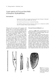
A new species of Cercyon from India (Coleoptera: Hydrophilidae)
Greek Government Gazette: Part 2, 2006 no. 510
DTIC ADA495964: Foreign Military Sales Sole Source Exception: The Current USASAC Practice
Capital-Skill Complementarity and the Emergence of Labor Emancipation
DTIC ADA462136: Valet Services: Improving Hidden Servers with a Personal Touch
