How do we generate random variables? PDF
Preview How do we generate random variables?
2WB05 Simulation Lecture 8: Generating random variables Marko Boon http://www.win.tue.nl/courses/2WB05 January7,2013 Outline 2/36 1. How do we generate random variables? 2. Fitting distributions DepartmentofMathematicsandComputerScience Generating random variables 3/36 How do we generate random variables? • Sampling from continuous distributions • Sampling from discrete distributions DepartmentofMathematicsandComputerScience Continuous distributions 4/36 Inverse Transform Method Let the random variable X have a continuous and increasing distribution function F. Denote the inverse of F by F−1. Then X can be generated as follows: • Generate U from U(0,1); • Return X = F−1(U). If F is not continuous or increasing, then we have to use the generalized inverse function F−1(u) = min{x : F(x) ≥ u}. DepartmentofMathematicsandComputerScience Continuous distributions 5/36 Examples • X = a + (b − a)U is uniform on (a,b); • X = −ln(U)/λ is exponential with parameter λ; • X = (−ln(U))1/a/λ is Weibull, parameters a and λ. Unfortunately, for many distribution functions we do not have an easy-to-use (closed-form) expression for the inverse of F. DepartmentofMathematicsandComputerScience Continuous distributions 6/36 Composition method This method applies when the distribution function F can be expressed as a mixture of other distribution func- , ,... tions F F , 1 2 ∞ (cid:88) F(x) = p F (x), i i i=1 ∞ where (cid:88) p ≥ 0, p = 1 i i i=1 The method is useful if it is easier to sample from the F ’s than from F. i • First generate an index I such that P(I = i) = p , i = 1,2,... i • Generate a random variable X with distribution function F . I DepartmentofMathematicsandComputerScience Continuous distributions 7/36 Examples • Hyper-exponential distribution: F(x) = p F (x) + p F (x) + ··· + p F (x), x ≥ 0, 1 1 2 2 k k where F (x) is the exponential distribution with parameter µ , i = 1,...,k. i i • Double-exponential (or Laplace) distribution: 1ex, x < 0; 2 f (x) = 1e−x, x ≥ 0, 2 where f denotes the density of F. DepartmentofMathematicsandComputerScience Continuous distributions 8/36 Convolution method ,..., In some case X can be expressed as a sum of independent random variables Y Y , so 1 n X = Y + Y + ··· + Y . 1 2 n where the Y ’s can be generated more easily than X. i Algorithm: • Generate independent Y ,...,Y , each with distribution function G; 1 n • Return X = Y + ··· + Y . 1 n DepartmentofMathematicsandComputerScience Continuous distributions 9/36 Example µ If X is Erlang distributed with parameters n and , then X can be expressed as a sum of n independent /µ exponentials Y , each with mean 1 . i Algorithm: • Generate n exponentials Y ,...,Y , each with 1 n µ mean ; • Set X = Y + ··· + Y . 1 n More efficient algorithm: • Generate n uniform (0,1) random variables ,..., U U ; 1 n • Set X = −ln(U U ···U )/µ. 1 2 n DepartmentofMathematicsandComputerScience Continuous distributions 10/36 Acceptance-Rejection method Denote the density of X by f . This method requires a function g that majorizes f , g(x) ≥ f (x) for all x. Now g will not be a density, since (cid:90) ∞ c = g(x)dx ≥ 1. −∞ Assume that c < ∞. Then h(x) = g(x)/c is a density. Algorithm: 1. Generate Y having density h; ( , ) 2. Generate U from U 0 1 , independent of Y; 3. If U ≤ f (Y)/g(Y), then set X = Y; else go back to step 1. The random variable X generated by this algorithm has density f . DepartmentofMathematicsandComputerScience
Description:The list of books you might like

As Good as Dead

Credence

Better Than the Movies

The Subtle Art of Not Giving a F*ck
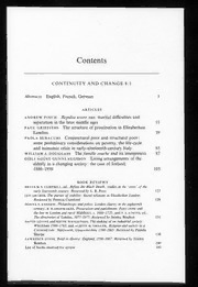
Continuity and Change 1993: Vol 8 Table of Contents
Geoderma 2006: Vol 136 Table of Contents

Marlinspike Sailor’s Knots and Crafts
By Kristin E. Anderson

Dünkirchen 1940: The German View of Dunkirk

El cerebro de Buda

Pablo Escobar em flagrante

Commencement
Commencement Exercises December 2006

by order of the commander air force materiel command air force
by (Under the Direction of AMIT SHETH) Workflow management

Avertissements Agricoles - Grandes cultures - Ile de France - 2006 - 13
DTIC ADA521948: Optics, Acoustics, and Stress in a Nearshore Bottom Nepheloid Layer
DTIC ADA521957: Vertical and Horizontal Migrations Affect Local and Integrated Water-Column Scattering Strengths
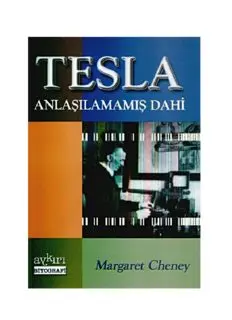
Tesla Anlaşılamamıs Dahi
Greek Government Gazette: Part 2, 2006 no. 551
Greek Government Gazette: Part 9, 2009 no. 52
